Restricted Distance Calculation

Partition Requirements

Our street network graph \(G = (V, E, l)\) with edges \(e \in E\) and vertices \(v \in V\) has a partition \(\mathcal{P} : G \mapsto \left(G_\mathrm{sp} \cup G_1 \cup \dots \cup G_k\right)\) returning subgraphs \(G_i\subseteq G\).

For a valid partitioning we want to calculate the distances and predecessors between all nodes while respecting the restrictions of the partitioning. The restrictions are that on a path it is only allowed once to leave and enter a partition.

We will guide through the idea of the algorithm in the following sections.

Small example

from itertools import combinations

import networkx as nx
import numpy as np
import pandas as pd
from matplotlib import pyplot as plt
from scipy.sparse import csr_matrix
from scipy.sparse.csgraph import dijkstra

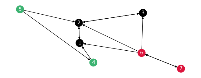
Imagine we have a directed graph with \(G_s, G_1, G_2\) as partitions and the following edges:

Show code cell source Hide code cell source

# Create graph
G = nx.DiGraph(
    [
        (1, 2, {"weight": 1}),
        (2, 1, {"weight": 1}),
        (2, 3, {"weight": 1}),
        (3, 2, {"weight": 1}),
        (1, 4, {"weight": 1}),
        (4, 1, {"weight": 1}),
        (2, 5, {"weight": 1}),
        (5, 2, {"weight": 1}),
        (5, 4, {"weight": 4}),
        (2, 4, {"weight": 1}),
        (3, 6, {"weight": 2}),
        (6, 3, {"weight": 2}),
        (6, 1, {"weight": 1}),
        (6, 2, {"weight": 6}),
        (6, 7, {"weight": 1}),
        (7, 6, {"weight": 1}),
        (6, 4, {"weight": 1.5}),
        (4, 6, {"weight": 1.5}),
    ]
)
# Draw a scaled down version of the graph
nx.draw(
    G,
    with_labels=True,
    font_color="white",
    pos=nx.kamada_kawai_layout(G),
    ax=plt.figure(figsize=(8, 3)).gca(),
)

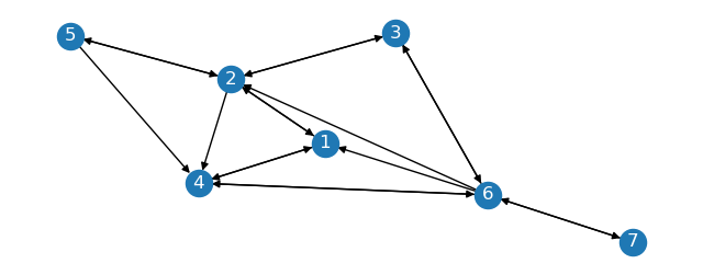
The sparse graph \(G_s\) is the subgraph of \(G\) with nodes \(1, 2, 3\).

n_sparse = [1, 2, 3]

The partitions \(G_1\) and \(G_2\) are the subgraphs of \(G\) with nodes \(4, 5\) and \(6\) respectively.

partitions = {
    "G_s": {"nodes": n_sparse, "color": "black", "subgraph": G.subgraph(n_sparse)},
    "G_1": {"nodes": [4, 5], "color": "mediumseagreen"},
    "G_2": {"nodes": [6, 7], "color": "crimson"},
}

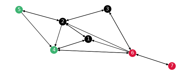
To each dictionary add a subgraph view, including all edges connecting to the nodes, and a node list with the connected nodes. Color the nodes according to the partition.

for name, part in partitions.items():
    if "subgraph" not in part:
        # subgraph for all edges from or to nodes in partition
        part["subgraph"] = G.edge_subgraph(
            [(u, v) for u, v in G.edges if u in part["nodes"] or v in part["nodes"]]
        )
    part["nodelist"] = part["subgraph"].nodes
    for node in part["nodes"]:
        G.nodes[node]["partition"] = part["color"]

nx.draw(G, with_labels=True, node_color=[G.nodes[n]["partition"] for n in G.nodes],
        font_color="white",
        pos=nx.kamada_kawai_layout(G),
        ax=plt.figure(figsize=(8,3)).gca(),
        )

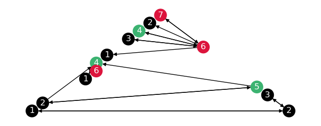
To check the subgraphs are correct, draw these separately.

# Copy subgraphs, relabel them, merge them into one graph
composite_graph = nx.DiGraph()
for name, part in partitions.items():
    subgraph = part["subgraph"].copy()
    subgraph = nx.relabel_nodes(subgraph, {n: f"{name}_{n}" for n in subgraph.nodes})
    composite_graph = nx.compose(composite_graph, subgraph)
nx.draw(
    composite_graph,
    node_color=[composite_graph.nodes[n]["partition"] for n in composite_graph.nodes],
    with_labels=True,
    font_color="white",
    labels={n: n.split("_")[-1] for n in composite_graph.nodes},
    pos=nx.planar_layout(composite_graph),
    ax=plt.figure(figsize=(8, 3)).gca(),
)

Distance calculation

To make the restricted calculation we use two passes of Dijsktra’s algorithm. One pass where it is only possible to leave the sparse graph and one pass where it is only possible to enter the sparse graph. Going between two partitions is always prohibited.

1. Leaving

Calculate all-pairs shortest paths on graph where we cut the edges that lead us outside a partition. This way we find all the shortest paths on the sparse graph, to one partition and inside all the partitions, without exiting. Also the edges between two different partitions are all cut.

2. Entering

Analogous to the first pass, but now we cut the edges that lead us into a partition. Here we will find the paths from partition nodes to the sparse graph nodes.

For finding the shortest paths we could use nx.floyd_warshall_predecessor_and_distance(), but as we’ll use this approach for larger graphs, we’ll use scipy.sparse.csgraph.dijkstra().

We will convert the graph to a sparse representation (csr) and filter out the concerning edges.

Show code cell source Hide code cell source

# sorted node order (names)
node_order = list(sorted(G.nodes))
# node_order indices
node_order_indices = list(range(len(node_order)))
# filtered indices: sparse/partition
n_sparse_indices = [node_order.index(n) for n in n_sparse]
part_name_order = [name for name in partitions.keys() if name != "G_s"]
n_partition_indices_separate = [
    [node_order.index(n) for n in partitions[name]["nodes"]] for name in part_name_order
]
n_partition_indices = [n for part in n_partition_indices_separate for n in part]
# Semipermeable graphs
G_leaving = G.copy()
# Construct Compressed Sparse Row matrix
# https://docs.scipy.org/doc/scipy/reference/generated/scipy.sparse.coo_matrix.html
G_leaving = nx.to_scipy_sparse_array(G_leaving, nodelist=node_order, format="coo")
data, row, col = G_leaving.data, G_leaving.row, G_leaving.col

# Remove edges between different partitions
# (col, row in separate n_partition_indices_separate)
for n_ind_1, n_ind_2 in combinations(n_partition_indices_separate, 2):
    mask = np.logical_and(np.isin(row, n_ind_1), np.isin(col, n_ind_2))
    mask = np.logical_or(mask,
                         np.logical_and(np.isin(row, n_ind_2), np.isin(col, n_ind_1)))
    data, row, col = data[~mask], row[~mask], col[~mask]
G_entering = (data, (row, col))

# Remove edges from partition to sparse
mask = np.logical_and(np.isin(row, n_partition_indices),
                      np.isin(col, n_sparse_indices))
data, row, col = data[~mask], row[~mask], col[~mask]
G_leaving = csr_matrix((data, (row, col)), shape=(len(node_order), len(node_order)))
# Remove edges from sparse to partition
data, (row, col) = G_entering
mask = np.logical_and(np.isin(row, n_sparse_indices),
                      np.isin(col, n_partition_indices))
data, row, col = data[~mask], row[~mask], col[~mask]
G_entering = csr_matrix((data, (row, col)), shape=(len(node_order), len(node_order)))

This will make the graph break up like so:

Show code cell source Hide code cell source

G_leaving_nx = nx.from_scipy_sparse_array(G_leaving, create_using=nx.DiGraph)
G_leaving_nx = nx.relabel_nodes(G_leaving_nx,
                                {i: n for i, n in enumerate(node_order)})
nx.draw(G_leaving_nx,
        with_labels=True,
        node_color=[G.nodes[n]["partition"] for n in G.nodes],
        font_color="white",
        pos=nx.kamada_kawai_layout(G_leaving_nx),
        ax=plt.figure(figsize=(8, 3)).gca(),
        )

Show code cell source Hide code cell source

G_entering_nx = nx.from_scipy_sparse_array(G_entering, create_using=nx.DiGraph)
G_entering_nx = nx.relabel_nodes(G_entering_nx,
                                 {i: n for i, n in enumerate(node_order)})
nx.draw(G_entering_nx,
        with_labels=True,
        node_color=[G.nodes[n]["partition"] for n in G.nodes],
        font_color="white",
        pos=nx.kamada_kawai_layout(G_entering_nx),
        ax=plt.figure(figsize=(8, 3)).gca(),
        )

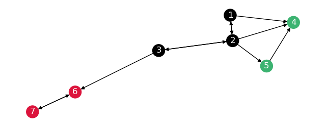
The distances on both these graphs are the following:

# Calculate distances on this graph
dist_leaving, pred_leaving = dijkstra(G_leaving, directed=True,
                                      return_predecessors=True)
dist_entering, pred_entering = dijkstra(G_entering, directed=True,
                                        return_predecessors=True)

display(pd.DataFrame(dist_leaving, index=node_order, columns=node_order),
        pd.DataFrame(dist_entering, index=node_order, columns=node_order))

	1	2	3	4	5	6	7
1	0.0	1.0	2.0	1.0	2.0	4.0	5.0
2	1.0	0.0	1.0	1.0	1.0	3.0	4.0
3	2.0	1.0	0.0	2.0	2.0	2.0	3.0
4	inf	inf	inf	0.0	inf	inf	inf
5	inf	inf	inf	4.0	0.0	inf	inf
6	inf	inf	inf	inf	inf	0.0	1.0
7	inf	inf	inf	inf	inf	1.0	0.0

	1	2	3	4	5	6	7
1	0.0	1.0	2.0	inf	inf	inf	inf
2	1.0	0.0	1.0	inf	inf	inf	inf
3	2.0	1.0	0.0	inf	inf	inf	inf
4	1.0	2.0	3.0	0.0	inf	inf	inf
5	2.0	1.0	2.0	4.0	0.0	inf	inf
6	1.0	2.0	2.0	inf	inf	0.0	1.0
7	2.0	3.0	3.0	inf	inf	1.0	0.0

Merge results

We can merge the distances and predecessors taking the minimum of the two distances.

Show code cell source Hide code cell source

def colored_predecessors(preds, graph=G, node_order=node_order,
                         node_order_indices=node_order_indices):
    return pd.DataFrame(preds, index=node_order_indices,
                        columns=node_order_indices).style. \
        map(lambda x: f"color: {graph.nodes[node_order[x]]['partition']}"
    if x != -9999 else "")


def colored_distances(dists, precision, cmap='Blues', node_order=node_order):
    return pd.DataFrame(dists, index=node_order, columns=node_order).style. \
        background_gradient(cmap=cmap, vmin=np.ma.masked_invalid(dists).min(),
                            vmax=np.ma.masked_invalid(dists).max()). \
        format(precision=precision)

min_mask = dist_leaving < dist_entering
dist_le = dist_entering.copy()
pred_le = pred_entering.copy()
dist_le[min_mask], pred_le[min_mask] = dist_leaving[min_mask], pred_leaving[min_mask]

display(colored_distances(dist_le, 1),
        colored_predecessors(pred_le))

	1	2	3	4	5	6	7
1	0.0	1.0	2.0	1.0	2.0	4.0	5.0
2	1.0	0.0	1.0	1.0	1.0	3.0	4.0
3	2.0	1.0	0.0	2.0	2.0	2.0	3.0
4	1.0	2.0	3.0	0.0	inf	inf	inf
5	2.0	1.0	2.0	4.0	0.0	inf	inf
6	1.0	2.0	2.0	inf	inf	0.0	1.0
7	2.0	3.0	3.0	inf	inf	1.0	0.0

	0	1	2	3	4	5	6
0	-9999	0	1	0	1	2	5
1	1	-9999	1	1	1	2	5
2	1	2	-9999	1	1	2	5
3	3	0	1	-9999	-9999	-9999	-9999
4	1	4	1	4	-9999	-9999	-9999
5	5	0	5	-9999	-9999	-9999	5
6	5	0	5	-9999	-9999	6	-9999

Predecessor Matrix

The predecessor matrix is used to reconstruct the shortest paths. Predecessor of \(i\) to \(j\) is the node with index \(k\) that is on the shortest path from \(i\) to \(j\). So the predecessor of \(i\) to \(j\) is \(k\) if \(d_{ij} = d_{ik} + d_{kj}\).

Now we know all the distances and paths if we only allow crossing to/from the sparsified graph once. The lower right corner of the matrices is still empty, as these are the paths between the partitions, which need to cross twice.

Fill up distances

For these all we will need to find the minimum of

\[ d_{ij} = \min_{k_n \in V_s\cup V_n, l_m \in V_s\cup V_m} \left(d_{ik} + d_{kl} + d_{lj}\right), \quad i \in V_n \Leftrightarrow j \in V_m\]

and the corresponding predecessor. But as we already now all the paths \(d_{ik} + d_{kl}\) entering, and \(d_{kl} + d_{lj}\) leaving, we can reduce the search to one node \(k_n\) or \(l_m\).

We will go with \(k_n\).

Show code cell source Hide code cell source

n_partition_intersect_indices = [
    list(set(n_sparse).intersection(partitions[name]["nodelist"]))
    for name in part_name_order
]
n_partition_intersect_indices = [
    [node_order.index(n) for n in part_indices]
    for part_indices in n_partition_intersect_indices
]

# Loop, for didactic purposes
for part_idx, part_intersect in zip(n_partition_indices_separate,
                                    n_partition_intersect_indices):
    for i in part_idx:
        for j in n_partition_indices:
            if i == j:
                continue
            # distances from i to j, over all possible k in part_intersect
            dists = dist_le[i, part_intersect] + dist_le[part_intersect, j]
            # index of minimum distance for predecessor
            min_idx = np.argmin(dists)
            if dists[min_idx] >= dist_le[i, j]:
                continue
            dist_le[i, j] = dists[min_idx]
            pred_le[i, j] = pred_le[part_intersect[min_idx], j]
# A vectorized version of the above is much quicker, see implementation

display(colored_distances(dist_le, 0),
        colored_predecessors(pred_le))

	1	2	3	4	5	6	7
1	0	1	2	1	2	4	5
2	1	0	1	1	1	3	4
3	2	1	0	2	2	2	3
4	1	2	3	0	3	5	6
5	2	1	2	2	0	4	5
6	1	2	2	2	3	0	1
7	2	3	3	3	4	1	0

	0	1	2	3	4	5	6
0	-9999	0	1	0	1	2	5
1	1	-9999	1	1	1	2	5
2	1	2	-9999	1	1	2	5
3	3	0	1	-9999	1	2	5
4	1	4	1	1	-9999	2	5
5	5	0	5	0	1	-9999	5
6	5	0	5	0	1	6	-9999

And there we already got our result. In this case the only difference results through the edge between \(6\) and \(4\), which is restricted. The shortest path differences are the following:

Show code cell source Hide code cell source

G_sparse = nx.to_scipy_sparse_array(G, nodelist=list(G.nodes))
G_sparse.indices, G_sparse.indptr = G_sparse.indices.astype(
    np.int32), G_sparse.indptr.astype(np.int32)
display(colored_distances(
    dist_le - dijkstra(G_sparse,
                       directed=True,
                       return_predecessors=False),
    1, 'Reds')
)

	1	2	3	4	5	6	7
1	0.0	0.0	0.0	0.0	0.0	1.5	1.5
2	0.0	0.0	0.0	0.0	0.0	0.5	0.5
3	0.0	0.0	0.0	0.0	0.0	0.0	0.0
4	0.0	0.0	0.0	0.0	0.0	3.5	3.5
5	0.0	0.0	0.0	0.0	0.0	0.5	0.5
6	0.0	0.0	0.0	0.5	0.0	0.0	0.0
7	0.0	0.0	0.0	0.5	0.0	0.0	0.0

To see a difference traversing the sparse graph, we will look at another example using the implementation of the algorithm in the package.

Second example

With the above described algorithm, the method shortest_paths_restricted() is implemented, see Implementation. It takes a graph and partitions as the input and returns the distance matrix and the predecessor matrix. Now we define the Graph G_2:

Show code cell source Hide code cell source

# Create planar graph, similar to a street network
G_2 = nx.DiGraph(nx.Graph(
    [
        (10, 11, {"weight": 1}),
        (11, 12, {"weight": 1}),
        (12, 13, {"weight": 1}),
        (13, 0, {"weight": 1.5}),
        (13, 14, {"weight": 1}),
        (14, 0, {"weight": 1}),
        (0, 10, {"weight": 1}),
        (0, 1, {"weight": 1}),
        (10, 1, {"weight": 1}),
        (1, 2, {"weight": 1}),
        (2, 3, {"weight": 1}),
        (3, 4, {"weight": 1.5}),
        (4, 5, {"weight": 1}),
        (5, 9, {"weight": 1}),
        (5, 6, {"weight": 1}),
        (7, 2, {"weight": 1}),
        (8, 7, {"weight": 0.5}),
        (7, 1, {"weight": 1}),
        (8, 9, {"weight": 0.7}),
        (6, 9, {"weight": 1}),
        (8, 4, {"weight": 1}),
        (9, 1, {"weight": 1}),
        (0, 18, {"weight": 0.4}),
        (18, 2, {"weight": 0.4}),
        (6, 15, {"weight": 0.8}),
        (15, 16, {"weight": 1}),
        (16, 17, {"weight": 1}),
        (17, 6, {"weight": 1}),
    ]
))
# Isolated node
G_2.add_node(19)
# Delete directed edges (1, 9), (6, 17), (10, 1)
G_2.remove_edges_from([(1, 9), (6, 17), (10, 1)])
# Add longer edge 0 -> 13
G_2.add_edge(0, 13, weight=G_2[0][13]["weight"] * 2)

n_sparse = [0, 1, 2, 3, 4, 5, 6, 19]
partitions = {
    "sparsified":
        {"nodes": n_sparse, "color": "black", "subgraph": G_2.subgraph(n_sparse)},
    "G_r": {"nodes": [7, 8, 9], "color": "crimson"},
    "G_g": {"nodes": [10, 11, 12, 13, 14], "color": "mediumseagreen"},
    "G_b": {"nodes": [15, 16, 17], "color": "dodgerblue"},
    "G_o": {"nodes": [18], "color": "darkorange"},
}
for name, part in partitions.items():
    if "subgraph" not in part:
        # subgraph for all edges from or to nodes in partition
        part["subgraph"] = G_2.edge_subgraph(
            [(u, v) for u, v in G_2.edges if u in part["nodes"] or v in part["nodes"]]
        )
    part["nodelist"] = part["subgraph"].nodes
    for node in part["nodes"]:
        G_2.nodes[node]["partition"] = part["color"]

nx.draw(G_2, with_labels=True, node_color=[G_2.nodes[n]["partition"] for n in G_2
        .nodes],
        font_color="white",
        pos=nx.kamada_kawai_layout(G_2),
        ax=plt.figure(figsize=(8, 5)).gca(),
        )

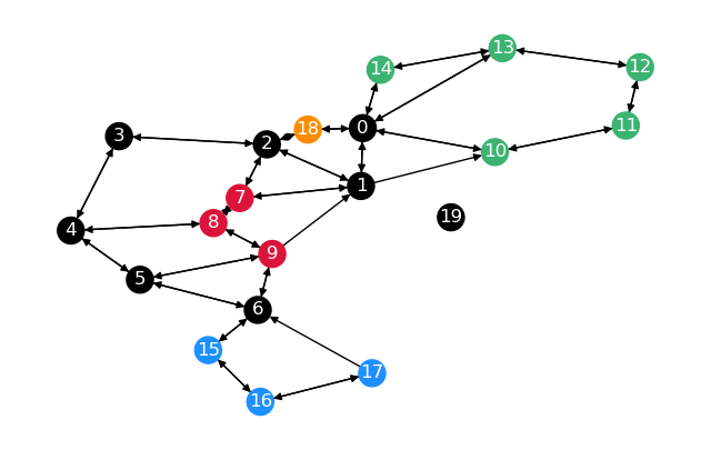
Two notes to this graph. The distance between \(0\) and \(2\) is \(0.8\) on the unrestricted graph \(0 \overset{0.4}{\rightarrow} 18 \overset{0.4}{\rightarrow} 2\), instead of \(2\) with restrictions \(0 \overset{1}{\rightarrow} 1 \overset{1}{\rightarrow} 2\). Getting from \(1\) to \(6\) would also be far shorter than taking the shortest path on the sparsified graph. The calculation using shortest_paths_restricted(G_2) gives the following results.

from superblockify.metrics.distances import shortest_paths_restricted

node_order_2 = list(range(len(G_2.nodes)))
dist, pred = shortest_paths_restricted(G_2, partitions, weight="weight",
                                       node_order=node_order_2)
display(colored_distances(dist, 1, node_order=node_order_2). \
        set_table_attributes('style="font-size: 12px"'),
        colored_predecessors(pred, G_2, node_order=node_order_2,
                             node_order_indices=node_order_2). \
        set_table_attributes('style="font-size: 10px"'))

2024-08-21 10:13:29,168 |     INFO | __init__.py:11 | superblockify version 1.0.0

	0	1	2	3	4	5	6	7	8	9	10	11	12	13	14	15	16	17	18	19
0	0.0	1.0	2.0	3.0	4.5	5.5	6.5	2.0	2.5	3.2	1.0	2.0	3.0	2.0	1.0	7.3	8.3	9.3	0.4	inf
1	1.0	0.0	1.0	2.0	3.5	4.5	5.5	1.0	1.5	2.2	1.0	2.0	3.0	3.0	2.0	6.3	7.3	8.3	1.4	inf
2	2.0	1.0	0.0	1.0	2.5	3.5	4.5	1.0	1.5	2.2	2.0	3.0	4.0	4.0	3.0	5.3	6.3	7.3	0.4	inf
3	3.0	2.0	1.0	0.0	1.5	2.5	3.5	2.0	2.5	3.2	3.0	4.0	5.0	5.0	4.0	4.3	5.3	6.3	1.4	inf
4	4.5	3.5	2.5	1.5	0.0	1.0	2.0	1.5	1.0	1.7	4.5	5.5	6.5	6.5	5.5	2.8	3.8	4.8	2.9	inf
5	5.5	4.5	3.5	2.5	1.0	0.0	1.0	2.2	1.7	1.0	5.5	6.5	7.5	7.5	6.5	1.8	2.8	3.8	3.9	inf
6	6.5	5.5	4.5	3.5	2.0	1.0	0.0	2.2	1.7	1.0	6.5	7.5	8.5	8.5	7.5	0.8	1.8	2.8	4.9	inf
7	2.0	1.0	1.0	2.0	1.5	2.2	2.2	0.0	0.5	1.2	2.0	3.0	4.0	4.0	3.0	3.0	4.0	5.0	1.4	inf
8	2.5	1.5	1.5	2.5	1.0	1.7	1.7	0.5	0.0	0.7	2.5	3.5	4.5	4.5	3.5	2.5	3.5	4.5	1.9	inf
9	2.0	1.0	2.0	3.0	1.7	1.0	1.0	1.2	0.7	0.0	2.0	3.0	4.0	4.0	3.0	1.8	2.8	3.8	2.4	inf
10	1.0	2.0	3.0	4.0	5.5	6.5	7.5	3.0	3.5	4.2	0.0	1.0	2.0	3.0	2.0	8.3	9.3	10.3	1.4	inf
11	2.0	3.0	4.0	5.0	6.5	7.5	8.5	4.0	4.5	5.2	1.0	0.0	1.0	2.0	3.0	9.3	10.3	11.3	2.4	inf
12	2.5	3.5	4.5	5.5	7.0	8.0	9.0	4.5	5.0	5.7	2.0	1.0	0.0	1.0	2.0	9.8	10.8	11.8	2.9	inf
13	1.5	2.5	3.5	4.5	6.0	7.0	8.0	3.5	4.0	4.7	2.5	2.0	1.0	0.0	1.0	8.8	9.8	10.8	1.9	inf
14	1.0	2.0	3.0	4.0	5.5	6.5	7.5	3.0	3.5	4.2	2.0	3.0	2.0	1.0	0.0	8.3	9.3	10.3	1.4	inf
15	7.3	6.3	5.3	4.3	2.8	1.8	0.8	3.0	2.5	1.8	7.3	8.3	9.3	9.3	8.3	0.0	1.0	2.0	5.7	inf
16	8.3	7.3	6.3	5.3	3.8	2.8	1.8	4.0	3.5	2.8	8.3	9.3	10.3	10.3	9.3	1.0	0.0	1.0	6.7	inf
17	7.5	6.5	5.5	4.5	3.0	2.0	1.0	3.2	2.7	2.0	7.5	8.5	9.5	9.5	8.5	1.8	1.0	0.0	5.9	inf
18	0.4	1.4	0.4	1.4	2.9	3.9	4.9	1.4	1.9	2.6	1.4	2.4	3.4	2.4	1.4	5.7	6.7	7.7	0.0	inf
19	inf	inf	inf	inf	inf	inf	inf	inf	inf	inf	inf	inf	inf	inf	inf	inf	inf	inf	inf	0.0

	0	1	2	3	4	5	6	7	8	9	10	11	12	13	14	15	16	17	18	19
0	-9999	0	1	2	3	4	5	1	7	8	0	10	11	14	0	6	15	16	0	-9999
1	1	-9999	1	2	3	4	5	1	7	8	1	10	11	14	0	6	15	16	0	-9999
2	1	2	-9999	2	3	4	5	2	7	8	1	10	11	14	0	6	15	16	2	-9999
3	1	2	3	-9999	3	4	5	2	4	8	1	10	11	14	0	6	15	16	2	-9999
4	1	2	3	4	-9999	4	5	8	4	8	1	10	11	14	0	6	15	16	2	-9999
5	1	2	3	4	5	-9999	5	8	9	5	1	10	11	14	0	6	15	16	2	-9999
6	1	2	3	4	5	6	-9999	8	9	6	1	10	11	14	0	6	15	16	2	-9999
7	1	7	7	2	8	9	9	-9999	7	8	1	10	11	14	0	6	15	16	2	-9999
8	1	7	7	4	8	9	9	8	-9999	8	1	10	11	14	0	6	15	16	2	-9999
9	1	9	1	2	8	9	9	8	9	-9999	1	10	11	14	0	6	15	16	0	-9999
10	10	0	1	2	3	4	5	1	7	8	-9999	10	11	12	0	6	15	16	0	-9999
11	10	0	1	2	3	4	5	1	7	8	11	-9999	11	12	13	6	15	16	0	-9999
12	13	0	1	2	3	4	5	1	7	8	11	12	-9999	12	13	6	15	16	0	-9999
13	13	0	1	2	3	4	5	1	7	8	0	12	13	-9999	13	6	15	16	0	-9999
14	14	0	1	2	3	4	5	1	7	8	0	12	13	14	-9999	6	15	16	0	-9999
15	1	2	3	4	5	6	15	8	9	6	1	10	11	14	0	-9999	15	16	2	-9999
16	1	2	3	4	5	6	15	8	9	6	1	10	11	14	0	16	-9999	16	2	-9999
17	1	2	3	4	5	6	17	8	9	6	1	10	11	14	0	6	17	-9999	2	-9999
18	18	0	18	2	3	4	5	2	7	8	0	10	11	14	0	6	15	16	-9999	-9999
19	-9999	-9999	-9999	-9999	-9999	-9999	-9999	-9999	-9999	-9999	-9999	-9999	-9999	-9999	-9999	-9999	-9999	-9999	-9999	-9999

At first glance the predecessor matrix looks correct. The yellow \(18\) is only predecessor coming from itself. Also for the red partition \(7\), \(8\), \(9\) we see that they are only being visited for the columns or rows corresponding to themselves. The same can be said for the other partitions. When going from or to sparsified nodes, no colorful nodes are visited.

From here one could reconstruct the shortest paths. A direct implementation for a single path would be the following.

def reconstruct_path(pred, start, end):
    """Reconstruct path from predecessor matrix."""
    if start == end:
        return []
    prev = pred[start]
    curr = prev[end]
    path = [end, curr]
    while curr != start:
        curr = prev[curr]
        path.append(curr)
    return list(reversed(path))

reconstruct_path(pred, 0, 2), reconstruct_path(pred, 0, 6), \
    reconstruct_path(pred, 14, 7), reconstruct_path(pred, 12, 16), \
    reconstruct_path(pred, 7, 18)

([0, 1, 2],
 [0, 1, 2, 3, 4, 5, 6],
 [14, 0, 1, 7],
 [12, 13, 0, 1, 2, 3, 4, 5, 6, 15, 16],
 [7, 2, 18])

Show code cell source Hide code cell source

nx.draw(G_2, with_labels=True, node_color=[G_2.nodes[n]["partition"] for n in G_2
        .nodes],
        font_color="white",
        pos=nx.kamada_kawai_layout(G_2),
        ax=plt.figure(figsize=(8, 5)).gca(),
        )

To finish, the difference between the unrestricted and restricted graph distances.

Show code cell source Hide code cell source

G_2_sparse = nx.to_scipy_sparse_array(G_2, nodelist=node_order_2)
G_2_sparse.indices, G_2_sparse.indptr = G_2_sparse.indices.astype(
    np.int32), G_2_sparse.indptr.astype(np.int32)
display(colored_distances(
    dist - dijkstra(G_2_sparse,
                    directed=True,
                    return_predecessors=False),
    1, 'Reds', node_order=node_order_2). \
        set_table_attributes('style="font-size: 12px"'),
        )

/tmp/ipykernel_2382/1105399673.py:5: RuntimeWarning: invalid value encountered in subtract
  dist - dijkstra(G_2_sparse,

	0	1	2	3	4	5	6	7	8	9	10	11	12	13	14	15	16	17	18	19
0	0.0	0.0	1.2	1.2	1.2	1.5	2.5	0.2	0.2	0.2	0.0	0.0	0.0	0.0	0.0	2.5	2.5	2.5	0.0	nan
1	0.0	0.0	0.0	0.0	1.0	1.3	2.3	0.0	0.0	0.0	0.0	0.0	0.0	0.0	0.0	2.3	2.3	2.3	0.0	nan
2	1.2	0.0	0.0	0.0	0.0	0.3	1.3	0.0	0.0	0.0	0.2	0.2	0.2	1.2	1.2	1.3	1.3	1.3	0.0	nan
3	1.2	0.0	0.0	0.0	0.0	0.0	0.0	0.0	0.0	0.0	0.2	0.2	0.2	1.2	1.2	0.0	0.0	0.0	0.0	nan
4	1.2	1.0	0.0	0.0	0.0	0.0	0.0	0.0	0.0	0.0	1.0	1.0	1.0	1.2	1.2	0.0	0.0	0.0	0.0	nan
5	2.5	2.5	0.5	0.0	0.0	0.0	0.0	0.0	0.0	0.0	2.5	2.5	2.5	2.5	2.5	0.0	0.0	0.0	0.5	nan
6	3.5	3.5	1.5	0.0	0.0	0.0	0.0	0.0	0.0	0.0	3.5	3.5	3.5	3.5	3.5	0.0	0.0	0.0	1.5	nan
7	0.2	0.0	0.0	0.0	0.0	0.0	0.0	0.0	0.0	0.0	0.0	0.0	0.0	0.2	0.2	0.0	0.0	0.0	-0.0	nan
8	0.2	0.0	0.0	0.0	0.0	0.0	0.0	0.0	0.0	0.0	0.0	0.0	0.0	0.2	0.2	0.0	0.0	0.0	-0.0	nan
9	0.0	0.0	0.0	0.0	0.0	0.0	0.0	0.0	0.0	0.0	0.0	0.0	0.0	0.0	0.0	-0.0	-0.0	-0.0	0.0	nan
10	0.0	0.0	1.2	1.2	1.2	1.5	2.5	0.2	0.2	0.2	0.0	0.0	0.0	0.0	0.0	2.5	2.5	2.5	-0.0	nan
11	0.0	0.0	1.2	1.2	1.2	1.5	2.5	0.2	0.2	0.2	0.0	0.0	0.0	0.0	0.0	2.5	2.5	2.5	0.0	nan
12	0.0	0.0	1.2	1.2	1.2	1.5	2.5	0.2	0.2	0.2	0.0	0.0	0.0	0.0	0.0	2.5	2.5	2.5	0.0	nan
13	0.0	0.0	1.2	1.2	1.2	1.5	2.5	0.2	0.2	0.2	0.0	0.0	0.0	0.0	0.0	2.5	2.5	2.5	-0.0	nan
14	0.0	0.0	1.2	1.2	1.2	1.5	2.5	0.2	0.2	0.2	0.0	0.0	0.0	0.0	0.0	2.5	2.5	2.5	-0.0	nan
15	3.5	3.5	1.5	0.0	0.0	0.0	0.0	0.0	0.0	-0.0	3.5	3.5	3.5	3.5	3.5	0.0	0.0	0.0	1.5	nan
16	3.5	3.5	1.5	0.0	0.0	0.0	0.0	0.0	0.0	-0.0	3.5	3.5	3.5	3.5	3.5	0.0	0.0	0.0	1.5	nan
17	3.5	3.5	1.5	0.0	0.0	0.0	0.0	0.0	0.0	0.0	3.5	3.5	3.5	3.5	3.5	-0.0	0.0	0.0	1.5	nan
18	0.0	0.0	0.0	0.0	0.0	0.3	1.3	-0.0	-0.0	-0.0	-0.0	0.0	0.0	0.0	-0.0	1.3	1.3	1.3	0.0	nan
19	nan	nan	nan	nan	nan	nan	nan	nan	nan	nan	nan	nan	nan	nan	nan	nan	nan	nan	nan	0.0

Implementation

superblockify.metrics.distances.calculate_partitioning_distance_matrix(partitioner, weight=None, unit_symbol=None, node_order=None, plot_distributions=False, check_overlap=True, max_mem_factor=0.2)

Calculate the distance matrix for the partitioning.

This is the pairwise distance between all pairs of nodes, where the shortest paths are only allowed to traverse edges in the start and goal partitions and unpartitioned edges. For this we calculate the distances and predecessors on the sparsified graph and the subgraphs separately. Then we combine the distances and predecessors to get a full distance matrix. We cannot do one big calculation, because the restrictions, to only enter/leave, are dynamic and depend on the start and goal node.

Parameters:

partitionerBasePartitioner

The partitioner to calculate the distance matrix for

weightstr, optional

The edge attribute to use as weight. If None, all edges have weight 1.

unit_symbolstr, optional

The unit symbol to use for the weight.

node_orderlist, optional

The order of the nodes in the distance matrix. If None, the ordering is produced by graph.nodes().

plot_distributionsbool, optional

If True, plot the distributions of the Euclidean distances and coordinates.

check_overlapbool, optional

If True, check that the partitions do not overlap node-wise.

max_mem_factorfloat, optional

The maximal memory factor to use for filling up the restricted distance matrices as tensor. Otherwise, using vectorized version.

Returns:

dist_matrixndarray

The distance matrix for the partitioning. dist_matrix[i, j] is the distance between node i and node j for the given rules of the partitioning. In the order of node_order if given, otherwise as produced by graph.nodes().

predecessorsndarray

The predecessor matrix for the partitioning. predecessors[i, j] is the predecessor of node j on the shortest path from node i for the given rules of the partitioning.

Raises:

ValueError

If partitions don’t have unique names.

ValueError

If the partitions overlap node-wise. For nodes considered to be in the partition, see BasePartitioner.get_partition_nodes().

superblockify.metrics.distances.shortest_paths_restricted(graph, partitions, weight, node_order, max_mem_factor=0.2)

Calculate restricted shortest paths.

Shortest distances and predecessors with restrictions of not passing through partitions. The passed partitions is a dictionary with the partition names as keys and the partition as value. The partition is a dictionary with the keys subgraph, nodes and nodelist. The dict needs to have a special partition, called sparsified, which is the sparsified graph. The nodes key is a list of nodes that are exclusive to the partition, i.e. nodes that are not shared with the sparsified graph or on partition boundaries. The nodelist key is a list of nodes that are exclusive to the partition and nodes that are shared with the sparsified graph. The subgraphs all need to be graphs views of a shared graph. The Partitioner class produces such partitions, after passing the integrated is_valid_partitioning() checks.

Parameters:

graphnetworkx.MultiDiGraph

The graph to calculate the shortest paths for.

partitionsdict

The partitions to calculate the shortest paths for. The keys are the partition names and the values are dictionaries with the keys subgraph, nodes and nodelist.

weightstr or None, optional

The edge attribute to use as weight. If None, all edge weights are 1.

node_orderlist

The order of the nodes in the distance matrix.

max_mem_factorfloat, optional

The maximum fraction to use in the fully vectorized calculation. Defaults to 0.2. Otherwise, the calculation is iterated over the partition indices.

Returns:

dist_matrixndarray

The distance matrix for the partitioning.

pred_matrixndarray

The predecessor matrix for the partitioning.

Notes

For usage with a Partitioner, see calculate_partitioning_distance_matrix().