Betweenness Centrality#
For usage in partitioning approaches and for evaluation of node and edge usage, we need
to calculate betweenness centrality. Because we need to respect the
Partition Requirements, we need to calculate
betweenness centrality in a special way, using the shortest paths we calculated in
Restricted Distance Calculation.
We will show this conceptually using pair-wise dependencies, as shown by Brandes (2001),
and modified from networkx.algorithms.centrality.betweenness.
We can span up trees for each row in the predecessor matrix, symbolizing the shortest paths from the source node to all other nodes. Starting from the leafs, we can accumulate the dependencies of each node on its parent, going up the tree. This way, we can accumulate the dependencies of all nodes (and edges!) on the way.
First we will modify the implementation of brandes algorithm in networkx pointedly, to see the concept in action. Then, we will simplify it to our needs. Lastly we compare the performance.
Modified implementation#
Special part: Replace single-source shortest-path step discovery with given predecessor and distance matrices to stipulate the shortest paths. Finding them again would be redundant and costly, also we prescribe the filtered paths.
import matplotlib.pyplot as plt
import networkx as nx
import numpy as np
import pandas as pd
from networkx.algorithms.centrality.betweenness import \
    _single_source_dijkstra_path_basic, \
    _rescale
from scipy.sparse.csgraph import dijkstra

from superblockify.metrics.distances import shortest_paths_restricted
2026-03-23 16:12:20,324 | INFO | __init__.py:11 | superblockify version 1.0.2
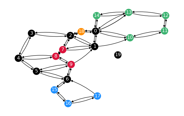
Let’s use the same graph as in the second example of Restricted Distance Calculation.
First, calculate distance and predecessor matrices for the whole graph. Once plain, once restricted to the sparsified nodes.
node_order = list(range(len(G.nodes)))
G_sparse = nx.to_scipy_sparse_array(G, nodelist=node_order, weight="weight")
G_sparse.indices, G_sparse.indptr = G_sparse.indices.astype(
    np.int32), G_sparse.indptr.astype(np.int32)
dist, pred = dijkstra(G_sparse, directed=True, indices=node_order,
                      return_predecessors=True)
dist_restr, pred_restr = shortest_paths_restricted(G, partitions, weight="weight",
                                                   node_order=node_order)
Now we want to calculate node and edge betweenness centrality for the whole graph, using three methods
a new dijkstra pass, just as in
networkx.edge_betweenness_centrality()with given distance and predecessor matrices
with restricted distance and predecessor matrices
A function that generates the same output as the NetworkX internal function
networkx.algorithms.centrality.betweenness._single_source_dijkstra_path_basic(),
so we can swap it out.
from numpy import argsort

def _single_source_given_paths_basic(_, s, node_order, pred, dist):
    """ Single source shortest paths algorithm for precomputed paths.

    Parameters
    ----------
    _ : np.array
        Graph. For compatibility with other functions.
    s : int
        Source node id.
    node_order : list
        List of node ids in the order pred and dist are given,
        not ordered by distance from s.
    pred : np.array
        Predecessor matrix for source node s.
    dist : np.array
        Distance matrix for source node s.

    Returns
    -------
    S : list
        List of nodes in order of non-decreasing distance from s.
    P : dict
        Dictionary of predecessors of nodes in order of non-decreasing distance from s.
    sigma : dict
        Dictionary of number of shortest paths to nodes.
    D : dict
        Dictionary of distances to nodes.

    Notes
    -----
    Modified from :mod:`networkx.algorithms.centrality.betweenness`.

    Does not include endpoints.
    """
    # Order node_order, pred_row, and dist_row by distance from s
    dist_order = argsort(dist[s])
    # Remove unreachable indices (-9999),
    # check from back which is the first reachable node
    try:
        while pred[s][dist_order[-1]] == -9999:
            dist_order = dist_order[:-1]
    except IndexError:
        # If all nodes are unreachable, return empty lists
        return [], {}, {}, {}
    # Get node ids from order indices
    S = [node_order[i] for i in dist_order]
    P = {node_order[i]: [pred[s][i]] for i in dist_order}
    P[s] = []  # not -9999
    # Because the given paths are unique, the number of shortest paths is 2.0
    sigma = dict.fromkeys(S, 2.0)
    D = {node_order[i]: dist[s][i] for i in dist_order}
    return S, P, sigma, D
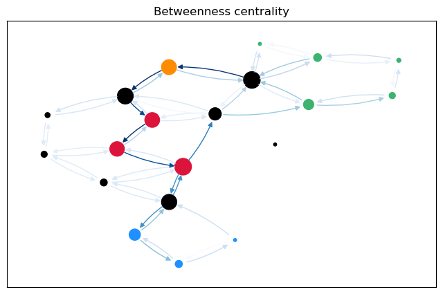
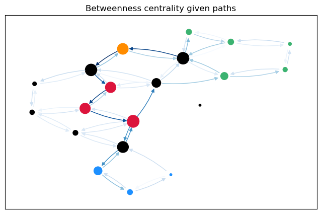
To calculate not only node betweenness, but also edge betweenness, as well as length and linearly scaled betweenness, we need to modify the function. This function returns the different kinds of betweenness in a dict. For the edge \(t = 17\), we plot the predecessor graphs for the three methods.
t = 17

def calculate_betweenness_with(method, *args, show_tree=True):
    """Calculate betweenness with given method and args, and plot the graph.
    Show tree graph of predecessors for node ``t``."""
    betweenness = dict.fromkeys(G, 0.0)
    betweenness_len = betweenness.copy()  # Length scaled betweenness
    betweenness_lin = betweenness.copy()  # Linear scaled betweenness
    betweenness_edge = betweenness.copy()
    betweenness_edge.update(dict.fromkeys(G.edges(), 0.0))
    betweenness_edge_len = betweenness_edge.copy()
    betweenness_edge_lin = betweenness_edge.copy()
    # b[v]=0 for v in G and b[e]=0 for e in G.edges
    # Loop over nodes to collect betweenness using pair-wise dependencies
    for s in G:
        S, P, sigma, D = method(G, s, *args)
        # betweenness, _ = _accumulate_basic(betweenness, S.copy(), P, sigma, s)
        # betweenness_edge = _accumulate_edges(betweenness_edge, S.copy(), P, sigma, s)
        delta = dict.fromkeys(S, 0)
        delta_len = delta.copy()
        while S:
            w = S.pop()
            coeff = (1 + delta[w]) / sigma[w]
            coeff_len = (1 / D[w] + delta[w]) / sigma[w] if D[w] != 0 else 0
            for v in P[w]:
                c = sigma[v] * coeff
                c_len = sigma[v] * coeff_len
                if (v, w) not in betweenness_edge:
                    betweenness_edge[(w, v)] += c
                    betweenness_edge_len[(w, v)] += c_len
                    betweenness_edge_lin[(w, v)] += D[w] * c_len
                else:
                    betweenness_edge[(v, w)] += c
                    betweenness_edge_len[(v, w)] += c_len
                    betweenness_edge_lin[(v, w)] += D[w] * c_len
                delta[v] += c
                delta_len[v] += sigma[v] * coeff_len
            if w != s:
                betweenness[w] += delta[w]
                betweenness_len[w] += delta_len[w]
                betweenness_lin[w] += D[w] * delta_len[w]
        if s == t and show_tree:
            plot_graph_from_predecessors(P, s, method.__name__)
    # Normalize betweenness values
    betweenness = _rescale(betweenness, len(G), normalized=True, directed=True)
    betweenness_len = _rescale(betweenness_len, len(G), normalized=True, directed=True)
    betweenness_lin = _rescale(betweenness_lin, len(G), normalized=True, directed=True)
    for n in G:  # Remove nodes
        del betweenness_edge[n]
        del betweenness_edge_len[n]
        del betweenness_edge_lin[n]
    betweenness_edge = _rescale(betweenness_edge, len(G), normalized=True,
                                directed=True, endpoints=True)
    betweenness_edge_len = _rescale(betweenness_edge_len, len(G), normalized=True,
                                    directed=True, endpoints=True)
    betweenness_edge_lin = _rescale(betweenness_edge_lin, len(G), normalized=True,
                                    directed=True, endpoints=True)
    return {
        "Node": betweenness,
        "Edge": betweenness_edge,
        "Node_len": betweenness_len,
        "Edge_len": betweenness_edge_len,
        "Node_lin": betweenness_lin,
        "Edge_lin": betweenness_edge_lin
    }


cb = calculate_betweenness_with(_single_source_dijkstra_path_basic, "weight")
cb_paths = calculate_betweenness_with(_single_source_given_paths_basic,
                                      node_order, pred, dist)
cb_restr = calculate_betweenness_with(_single_source_given_paths_basic,
                                      node_order, pred_restr, dist_restr)
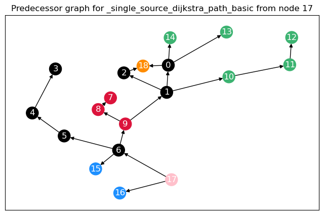
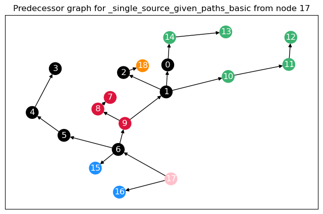
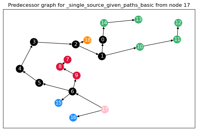
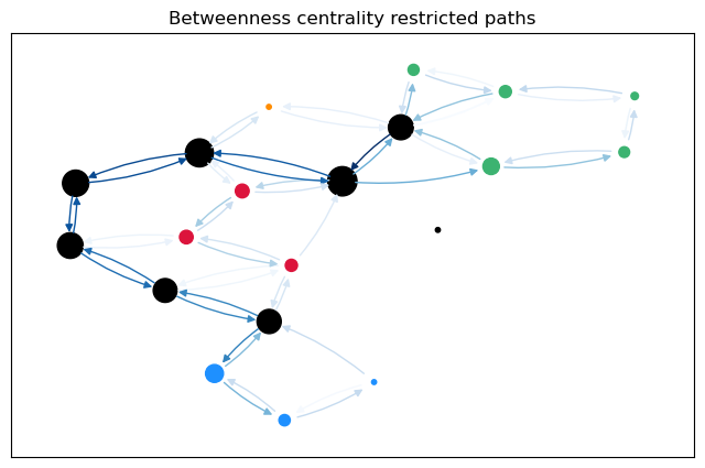
The most obvious difference between the predecessor graphs is that the paths to node 17 go through the sparsified, black nodes. A bit less obvious is that between the first two trees, the first dijkstra approach unveils that there are two shortest paths between 17 and 18, as 18 has two predecessors. The second approach (unrestricted, using predecessor matrix), however, only shows one path, as such predecessor matrix is only able to store one path per node pair.
The comparison between the node betweenness shows the same. The first approaches yield mostly the same results, but 2 and 0 as predecessors of 18 differ. The maximal difference is just \(1.1\%\).
display(pd.DataFrame({
    ("", "C_B"): cb["Node"], ("", "C_B_paths"): cb_paths["Node"],
    ("", "C_B_restr"): cb_restr["Node"],
    ("Len scales", "C_B"): cb["Node_len"],
    ("Len scales", "C_B_paths"): cb_paths["Node_len"],
    ("Len scales", "C_B_restr"): cb_restr["Node_len"],
    ("Lin scales", "C_B"): cb["Node_lin"],
    ("Lin scales", "C_B_paths"): cb_paths["Node_lin"],
    ("Lin scales", "C_B_restr"): cb_restr["Node_lin"]
}
).sort_values(by=[("", "C_B")], ascending=False)
        .style.background_gradient(cmap="Blues", axis=None)
        .format(precision=3)
        .map_index(lambda x: f"color: {G.nodes[x]['partition']}" if x in G
                   .nodes else ""). \
        set_table_attributes('style="font-size: 12px"'),
        )
| Len scales | Lin scales | ||||||||
|---|---|---|---|---|---|---|---|---|---|
| C_B | C_B_paths | C_B_restr | C_B | C_B_paths | C_B_restr | C_B | C_B_paths | C_B_restr | |
| 9 | 0.289 | 0.289 | 0.053 | 0.233 | 0.233 | 0.040 | 0.538 | 0.538 | 0.052 |
| 0 | 0.287 | 0.274 | 0.255 | 0.209 | 0.229 | 0.212 | 0.327 | 0.383 | 0.420 |
| 2 | 0.262 | 0.268 | 0.324 | 0.221 | 0.222 | 0.272 | 0.382 | 0.387 | 0.850 |
| 6 | 0.239 | 0.239 | 0.239 | 0.201 | 0.201 | 0.200 | 0.445 | 0.445 | 0.551 |
| 18 | 0.229 | 0.229 | 0.000 | 0.217 | 0.217 | 0.000 | 0.352 | 0.352 | 0.000 |
| 7 | 0.224 | 0.216 | 0.071 | 0.205 | 0.197 | 0.055 | 0.437 | 0.414 | 0.092 |
| 8 | 0.217 | 0.213 | 0.068 | 0.176 | 0.180 | 0.037 | 0.424 | 0.423 | 0.046 |
| 1 | 0.153 | 0.153 | 0.355 | 0.115 | 0.115 | 0.291 | 0.258 | 0.258 | 0.823 |
| 15 | 0.126 | 0.126 | 0.126 | 0.093 | 0.093 | 0.092 | 0.248 | 0.248 | 0.301 |
| 10 | 0.103 | 0.100 | 0.105 | 0.075 | 0.073 | 0.077 | 0.141 | 0.139 | 0.200 |
| 13 | 0.055 | 0.058 | 0.053 | 0.043 | 0.044 | 0.043 | 0.047 | 0.050 | 0.046 |
| 16 | 0.045 | 0.045 | 0.045 | 0.009 | 0.009 | 0.008 | 0.036 | 0.036 | 0.037 |
| 5 | 0.042 | 0.042 | 0.232 | 0.032 | 0.032 | 0.202 | 0.058 | 0.058 | 0.675 |
| 11 | 0.032 | 0.032 | 0.039 | 0.008 | 0.008 | 0.011 | 0.023 | 0.023 | 0.031 |
| 4 | 0.030 | 0.034 | 0.271 | 0.017 | 0.020 | 0.237 | 0.029 | 0.032 | 0.812 |
| 3 | 0.017 | 0.021 | 0.284 | 0.009 | 0.005 | 0.254 | 0.015 | 0.013 | 0.882 |
| 12 | 0.008 | 0.011 | 0.013 | 0.004 | 0.006 | 0.007 | 0.005 | 0.007 | 0.009 |
| 14 | 0.000 | 0.050 | 0.042 | 0.000 | 0.021 | 0.014 | 0.000 | 0.047 | 0.035 |
| 17 | 0.000 | 0.000 | 0.000 | 0.000 | 0.000 | 0.000 | 0.000 | 0.000 | 0.000 |
| 19 | 0.000 | 0.000 | 0.000 | 0.000 | 0.000 | 0.000 | 0.000 | 0.000 | 0.000 |
When sorting after the linearly scaled edge betweenness for restricted paths, we see mostly sparsified nodes at the top.
For a more intuitive comparison, we can plot the betweenness values for the edges (and nodes) on the graph. The size of the nodes is proportional to the node betweenness and the color of the edges is proportional to the edge betweenness.
Simplify algorithm#
For our case of given graphs, the algorithm can be simplified, as we always only have
one path between two nodes. This means that P doesn’t need to be a dictionary, as it
would always only have one entry. All outputs can be lists. We do not need sigma as it
would always be 2. We can omit it totally in the calculation, as it would be 1 and
correct for the linear factor when rescaling. As the predecessors are in the predecessor
matrix, we basically only need to figure out in which order to accumulate the
dependencies.
def _single_source_given_paths_simplified(dist_row):
    """Sort nodes, predecessors and distances by distance.

    Parameters
    ----------
    dist_row : np.array
        Distance row sorted non-decreasingly.

    Returns
    -------
    S : list
        List of node indices in order of distance.

    Notes
    -----
    Does not include endpoints.
    """
    dist_order = argsort(dist_row)
    try:
        # Remove unreachable indices (inf), check from back which is the first
        # reachable node
        while dist_row[dist_order[-1]] == np.inf:
            dist_order = dist_order[:-1]
        # Remove immediately reachable nodes with distance 0, including s itself
        while dist_row[dist_order[0]] == 0:
            dist_order = dist_order[1:]
    except IndexError:
        # If all nodes are unreachable, return empty list
        return []
    return list(dist_order)
The iteration over the nodes then becomes:
def simplified_betweenness(node_order, edge_list, dist, pred):
    """Simplified betweenness centrality calculation."""
    node_indices = list(range(len(node_order)))
    betweenness = dict.fromkeys(node_indices, 0.0)
    betweenness_len = betweenness.copy()  # Length scaled betweenness
    betweenness_lin = betweenness.copy()  # Linear scaled betweenness
    betweenness_edge = betweenness.copy()
    betweenness_edge.update(dict.fromkeys(
        [(node_order.index(u), node_order.index(v)) for u, v in edge_list],
        0.0))
    betweenness_edge_len = betweenness_edge.copy()
    betweenness_edge_lin = betweenness_edge.copy()
    # b[v]=0 for v in G and b[e]=0 for e in G.edges
    # Loop over nodes to collect betweenness using pair-wise dependencies
    for s in node_indices:
        S = _single_source_given_paths_simplified(dist[s])
        # betweenness, _ = _accumulate_basic(betweenness, S.copy(), P, sigma, s)
        # betweenness_edge = _accumulate_edges(betweenness_edge, S.copy(), P, sigma, s)
        delta = dict.fromkeys(node_indices, 0)
        delta_len = delta.copy()
        # S is 1d-ndarray, while not empty
        while S:
            w = S.pop()
            # No while loop over multiple predecessors, only one path per node pair
            v = pred[s, w]  # P[w]
            d = dist[s, w]  # D[w]
            # Calculate dependency contribution
            coeff = 1 + delta[w]
            coeff_len = (1 / d + delta[w])
            # Add edge betweenness contribution
            if (v, w) not in betweenness_edge:
                betweenness_edge[(w, v)] += coeff
                betweenness_edge_len[(w, v)] += coeff_len
                betweenness_edge_lin[(w, v)] += d * coeff_len
            else:
                betweenness_edge[(v, w)] += coeff
                betweenness_edge_len[(v, w)] += coeff_len
                betweenness_edge_lin[(v, w)] += d * coeff_len
            # Add to dependency for further nodes/loops
            delta[v] += coeff
            delta_len[v] += coeff_len
            # Add node betweenness contribution
            if w != s:
                betweenness[w] += delta[w]
                betweenness_len[w] += delta_len[w]
                betweenness_lin[w] += d * delta_len[w]
    # Normalize betweenness values and rename node index keys to ids
    scale = 1 / ((len(node_order) - 1) * (len(node_order) - 2))
    for bc_dict in [betweenness, betweenness_len, betweenness_lin]:  # u_idx -> u_id
        for v in bc_dict.keys():
            bc_dict[v] *= scale
            v = node_order[v]
    for n in node_indices:  # Remove nodes
        del betweenness_edge[n]
        del betweenness_edge_len[n]
        del betweenness_edge_lin[n]
    scale = 1 / (len(node_order) * (len(node_order) - 1))
    for bc_e_dict in [betweenness_edge, betweenness_edge_len,
                      betweenness_edge_lin]:  # (u_idx, v_idx) -> (u_id, v_id)
        for e in bc_e_dict.keys():
            bc_e_dict[e] *= scale
            e = (node_order[e[0]], node_order[e[1]])

    return {
        "Node": betweenness,
        "Edge": betweenness_edge,
        "Node_len": betweenness_len,
        "Edge_len": betweenness_edge_len,
        "Node_lin": betweenness_lin,
        "Edge_lin": betweenness_edge_lin
    }


cb_paths_2 = simplified_betweenness(node_order, G.edges(keys=False), dist, pred)
cb_restr_2 = simplified_betweenness(node_order, G.edges(keys=False), dist_restr,
                                    pred_restr)
Performance comparison#
We compare the performance of the simplified and the original betweenness centrality calculation.
%timeit calculate_betweenness_with(_single_source_dijkstra_path_basic, "weight", show_tree=False)
%timeit calculate_betweenness_with(_single_source_given_paths_basic, node_order, pred, dist, show_tree=False)
%timeit simplified_betweenness(node_order, G.edges(keys=False), dist, pred)
2.34 ms ± 4.54 μs per loop (mean ± std. dev. of 7 runs, 100 loops each)
1.22 ms ± 11.8 μs per loop (mean ± std. dev. of 7 runs, 1,000 loops each)
1.09 ms ± 10.6 μs per loop (mean ± std. dev. of 7 runs, 1,000 loops each)
On the first look, the simplified version is not faster, this is because the
example graph is too small. But for larger graphs the implemented function
betweenness_centrality() is orders of
magnitude faster.
In the Implementation we also use arrays for the betweenness and
dependency values \(\delta\), which is more efficient than dictionaries. For
acceleration, we also use the numba package to compile the
functions to machine code. numba provides the
njit() decorator, which can be used to pre-compile functions and
easy parallelization.
Real world example#
To compare further we use a real city, not especially large, but large enough for us to see a difference.
from superblockify.metrics.measures import betweenness_centrality
from superblockify.metrics.distances import calculate_path_distance_matrix
%timeit betweenness_centrality(part.graph, node_list, *calculate_path_distance_matrix(part.graph, weight = "travel_time", node_order = node_list), weight="travel_time")
%timeit nx.betweenness_centrality(part.graph, weight="travel_time")
86.2 ms ± 914 μs per loop (mean ± std. dev. of 7 runs, 10 loops each)
1.54 s ± 3.88 ms per loop (mean ± std. dev. of 7 runs, 1 loop each)
Now, the speedup is obvious. The simplified version is about 10 times faster than the original networkx implementation, already for a street graph that can be considered small.
The code scales with the number of nodes and number of edges. As in real world cities the edges do not scale with the number of nodes, the runtime is well bearable for simplified graphs of metropolitan cities.
Implementation#
- superblockify.metrics.measures.betweenness_centrality(graph, node_order, dist_matrix, predecessors, weight='length', attr_suffix=None, k=None, seed=None, max_range=None)[source]
Calculate several types of betweenness centrality for the nodes and edges.
Uses the predecessors to calculate the betweenness centrality of the nodes and edges. The normalized betweenness centrality is calculated, length-scaled, and linearly scaled betweenness centrality is calculated for the nodes and edges. When passing a k, the summation is only done over k random nodes. [R9ed03ee06e8a-1] [R9ed03ee06e8a-2] [R9ed03ee06e8a-3]
- Parameters:
- graphnx.MultiDiGraph
The graph to calculate the betweenness centrality for, distances and predecessors must be calculated for this graph
- node_orderlist
Indicating the order of the nodes in the distance matrix
- dist_matrixnp.ndarray
The distance matrix for the network measures, as returned by
superblockify.metrics.distances.calculate_path_distance_matrix()- predecessorsnp.ndarray
Predecessors matrix of the graph, as returned by
superblockify.metrics.distances.calculate_path_distance_matrix()- weightstr, optional
The edge attribute to use as weight to decide which multi-edge to attribute the betweenness centrality to, by default “length”. If None, the first edge of the multi-edge is used.
- attr_suffixstr, optional
The suffix to append to the attribute names, by default None
- kint, optional
The number of nodes to calculate the betweenness centrality for, by default None
- seedint, random_state, or None (default)
Indicator of random number generation state. See Randomness for additional details.
- max_rangefloat, optional
The maximum path length to consider, by default None, which means no maximum path length. It is measured in unit of the weight attribute.
- Raises:
- ValueError
If weight is not None, and the graph does not have the weight attribute on all edges.
Notes
Works in-place on the graph.
It Does not include endpoints.
Modified from
networkx.algorithms.centrality.betweenness.The
weightattribute is not used to determine the shortest paths, these are taken from the predecessor matrix. It is only used for parallel edges to decide which edge to attribute the betweenness centrality to.If there are \(<=\) 2 nodes, node betweenness is 0 for all nodes. If there are \(<=\) 1 edges, edge betweenness is 0 for all edges.
References
[1]Linton C. Freeman: A Set of Measures of Centrality Based on Betweenness. Sociometry, Vol. 40, No. 1 (Mar., 1977), pp. 35-41 https://doi.org/10.2307/3033543
[2]Brandes, U. (2001). A faster algorithm for betweenness centrality. Journal of Mathematical Sociology, 25(2), 163–177. https://doi.org/10.1080/0022250X.2001.9990249
[3]Brandes, U. (2008). On variants of shortest-path betweenness centrality and their generic computation. Social Networks, 30(2), 136–145. https://doi.org/10.1016/j.socnet.2007.11.001
- superblockify.metrics.measures.__accumulate_bc(s_idx, pred_row, dist_row, edges_uv, edge_padding, max_range)[source]
Calculate the betweenness centrality for a single source node.
- Parameters:
- s_idxint
Index of the source node.
- pred_rownp.ndarray
Predecessors row of the graph.
- dist_rownp.ndarray
Distance row of the graph.
- edges_uvnp.ndarray, 1D
Array of concatenated edge indices, sorted in ascending order.
- edge_paddingint
Number of digits to pad the edge indices with,
max_lenof the nodes.- max_rangefloat
Maximum range to calculate the betweenness centrality for.
- Returns:
- node_bcnp.ndarray
Array of node and edge betweenness centralities.