Street Tessellation#
In this notebook we show how the street tesselation is working and some of the process how we got there. See Implementation for a usage example and the function stubs. How the population is distributed is explained in the next notebook Street Population Density.
2026-03-23 16:15:29,265 | INFO | __init__.py:11 | superblockify version 1.0.2
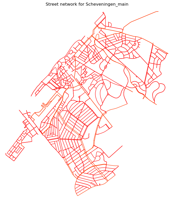
First we will get a partitioned city, namely Scheveningen. We can do this easily with
a superblockify partitioner.
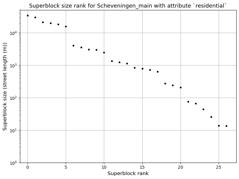
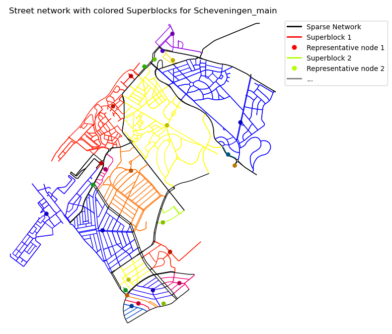
The partitioner has been run and for each Superblock it produces a partition, inclusing a subgraph object, which includes the nodes and edges of the Superblock. One of them looks like this:
subgraph = part.partitions[6]["subgraph"]
subgraph_edges = ox.graph_to_gdfs(subgraph, nodes=False, edges=True)
subgraph_edges.explore(style_kwds={"weight": 4})
As edges are represented by linestrings, the area is not clearly defined. The first idea that might come to one’s mind is the convex hull of the linestrings.
# From subgraph_edges we want to get a hull that encloses all edges
convex_hull = subgraph_edges.union_all().convex_hull
# Make gdf from convex hull with the same crs as the subgraph
convex_hull_gdf = gpd.GeoDataFrame(
    geometry=[convex_hull], crs=subgraph_edges.crs
)
# plot both gdfs together
ax = subgraph_edges.plot()
convex_hull_gdf.plot(ax=ax, color="lightgray")
plt.axis("off")
plt.show()
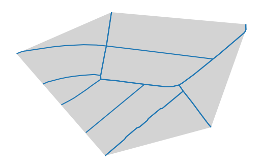
This approach is quick and easy, but it has some drawbacks. It might be larger than
we are looking for. For example, a star shaped neighborhood would result in a hull
spanning around all areas between the streets, even if it might include areas that
belong to another Superblock. Also, it might be smaller than we are looking for. For example,
a neighborhood that is linear, one long street with houses on both sides, would result
in a hull that is just a line, which is not what we are looking for.
The latter problem can be solved by buffering the edges before taking the convex hull.
The former problem has multiple solutions summarized under the term concave hull.
shapely provides the function
concave_hull for this purpose. It takes a ratio
parameter, which determines how concave the hull is. A ratio of 1 results in the convex
hull, a ratio of 0 results in only a line between the nearest points in the geometry.
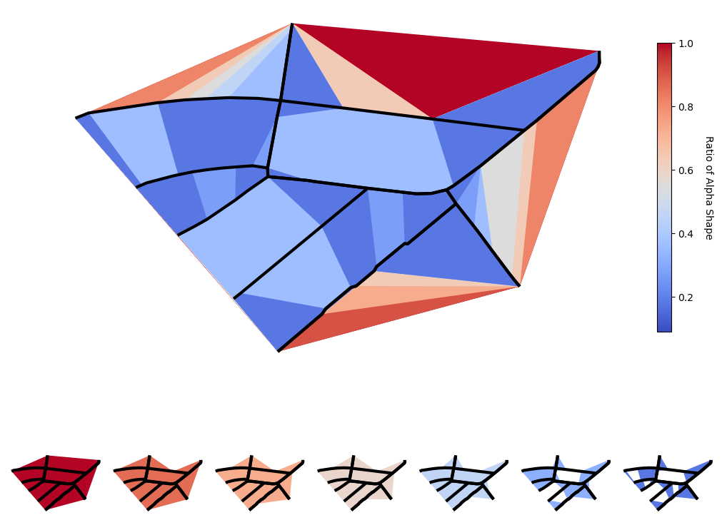
The function works with the points in the linestrings, so it is highly dependent on the point density. The ratio determines the maximum edge length, rescaled between the greatest and smallest distance between al pairs of points. This results in the fact, that a shape with lower ratio is not necessarily fully included in a shape with a higher ratio, see the two lowest ratios on the bottom right. This solution still does not satisfy us.
Optimally all Superblock cells would not overlap each other and form a tiling, also called tesselation, of the city.
Morphological Tessellation#
There is a solution satisfying our requirements. Okabe and Sugihara define the
line Network Voronoi Diagram (line N-VD) [Equation 4.7]. It is basically a Voronoi
diagram (also called Thiessen polygons in some fields) where lines are made up of
multiple points[1].
Araldi and Fusco use this idea to do geostatistical analysis[2]. Fleischmann et al.
implement the same idea in the momepy package for building footprints [3].
With list of footprint geometries, the Tessellation
class returns a GeoDataFrame with a cell corresponding to each input geometry that was
given.

In our case the input geometries can be the smaller neighborhood boundaries, and the tesselation fills up the gaps. For the Superblocks we will use an union of the edges of the subgraphs and buffer them a small bit. As we do not want the polygons to overlap wich each other, we’ll buffer using a flat cap style.
 def border_from_subgraph_shrinked(subgraph, buffer=1):
    """Shrinked subgraph borders, to avoid overlap between partitions.
    Does work well with small buffer values."""
    edges = ox.graph_to_gdfs(subgraph, nodes=False, edges=True)
    # First buffer with flat cap style to avoid self-intersections
    polygon = shp.Polygon(edges.union_all().buffer(2 * buffer, cap_style='flat')
                          .exterior)
    # Simplify the polygon to remove small artifacts of flat cap style at curved edges
    # polygon = polygon.simplify(buffer*2, preserve_topology=True)
    # geos::simplify::PolygonHullSimplifier would do the job. No bindings yet.
    # https://libgeos.org/doxygen/classgeos_1_1simplify_1_1PolygonHullSimplifier.html
    # http://lin-ear-th-inking.blogspot.com/2022/04/outer-and-inner-concave-polygon-hulls.html
    # http://lin-ear-th-inking.blogspot.com/2022/05/using-outer-hulls-for-smoothing.html
    # Secondly, erode the polygon to avoid overlap between partitions
    return polygon.buffer(-buffer, cap_style='round')

border_from_subgraph_shrinked(part.partitions[6]["subgraph"], buffer=1)
  Cell In[7], line 1
    def border_from_subgraph_shrinked(subgraph, buffer=1):
    ^
IndentationError: unexpected indent
We would like to simplify the polygon before buffering down, but as we use a flat
cap style, the line connection have small artifacts when choosing larger buffers.
The Ramer–Douglas–Peucker algorithm does not suffice our needs, because the result can
split the polygon up and does not inherently enclose the original polygon.
The geos::simplify::PolygonHullSimplifier would do the job, but it got added in GEOS
3.11, and no python package has any bindings, yet.
Now, when using the momepy.Tessellation class, we get:
from momepy import Tessellation

borders = gpd.GeoDataFrame(
    geometry=[border_from_subgraph_shrinked(p["subgraph"], buffer=1) for p in part
    .partitions],
    crs=part.partitions[0]["subgraph"].graph["crs"],
    data=[p["name"] for p in part.partitions],
    columns=["partition_id"]
)
# Morphological tessellation around given buildings ``gdf`` within set ``limit``.
tessellation = Tessellation(borders, unique_id="partition_id",
                               limit=part.graph.graph["boundary"],
                               shrink=0.0)
# Plot on our map
tessellation_gdf = tessellation.tessellation
fig, axe = plt.subplots(figsize=(10, 10))
tessellation_gdf.plot(ax=axe, edgecolor="white", column="partition_id", legend=True,
                      cmap="tab20")
borders.plot(ax=axe, color="white", alpha=0.5, facecolor="white")
ox.plot_graph(part.sparsified, ax=axe, node_size=0, edge_color="black",
              edge_linewidth=1)
axe.set_axis_off()
plt.show()
This is much more what we want. Another way to make it even better it so take the sparsified network at cell borders, but at the same time, the sparsified network should also have a volume as there might be people living on it. Finally, we will implement our own method, inspired by this technique, a solution sewed to our needs.
Independent Tessellation#
When looking into the code, momepy uses scipy.spatial.Voronoi
to generate the tessellation for every enclosure. This is done with a dense point array
for the geometry boundaries (borders in our case).
As we want to calculate area and population for each Partition, we can save time by
calculating the Voronoi diagram once for the whole graph/city, and save area and
population for each edge. Later we can use this data to calculate the area and
population for each Partition.
Now, we will create Voronoi cells for each edge, so we can later dissolve them to
Superblock cells. As we are working in a MultiDiGraph two way streets are represented by two
directed edges with the same geometry, both should share the same cell, so grouping the
edges is a crucial part. First we will group the edges connecting the same nodes u and
v and then we will merge the edges with the same or reverse geometry.
edges = ox.graph_to_gdfs(part.graph,
                         nodes=False,
                         edges=True,
                         node_geometry=False,
                         fill_edge_geometry=True)
# `edges` is a pandas dataframe with the multiindex (u, v, key)
# Merge two columns, when the geometry of one is equal or the reverse of the other
# 1. Group if u==u and v==v or u==v and v==u (match for hashed index (u, v) where u<v)
# get flat index of the first match
edges["edge_id"] = edges.index.to_flat_index()
# sort the edge_id tuples
edges["node_pair"] = edges["edge_id"].apply(lambda x: tuple(sorted(x[:2])))
# 2. Aggregate if the geometry is equal or the reverse of the other
# Merge columns if geometry_1 == geometry_2 or geometry_1 == geometry_2.reverse()
# reverse geometry if x_start >= x_end
edges["geometry"] = edges["geometry"].apply(
    lambda x: x if x.coords[0] < x.coords[-1] else x.reverse())
# 3. Group by node_pair and geometry
edges = edges.groupby(["node_pair", "geometry"]).agg({
    "edge_id": tuple,
    "component_name": "first",
}).reset_index()
edges.set_index("edge_id", inplace=True)

edges = gpd.GeoDataFrame(edges, geometry="geometry", crs=part.graph.graph["crs"])
edges.explore()
For each geometry we will interpolate the lines into points of equal distance of 10m.
# get multiindex of first row
distance = 10
# The maximum distance between points after discretization.
edge_points = []
edge_indices = []
# iterate over street_id, geometry
for idx, geometry in edges["geometry"].items():
    if geometry.length < 2 * distance:
        # for edges that would result in no point, take the middle
        pts = [shp.line_interpolate_point(geometry, 0.5, normalized=True)]
    else:
        # interpolate points along the line with at least distance between them
        # start and end 0.1 from the ends to avoid edge effects
        pts = shp.line_interpolate_point(
                geometry,
                np.linspace(
                    0.1,
                    geometry.length - 0.1,
                    num=int((geometry.length - 0.1) // distance),
                ),
            )  # offset to keep nodes out
    edge_points.append(shp.get_coordinates(pts))
    # Append multiindices for this geometry
    edge_indices += [idx] * len(pts)

points = np.vstack(edge_points)
Now we know for each point, which edge it belongs to. We can use this to calculate the Voronoi diagram.
Before we continue, let’s also introduce a hull around the points, so that the outer edge cells are not infinite or too large. As a hull we can use the boundary polygon of the graph from OSM, as used in the node approach, or a buffered union of the edge geometries. Then we can also split up the hull into points and add them to the points array.
hull = shp.Polygon(edges.union_all().buffer(100).exterior)
# interpolate points along the hull - double the distance
hull_points = shp.line_interpolate_point(
    hull.boundary,
    np.linspace(0.1, hull.length - 0.1, num=int(hull.length // (2 * distance))),
)
# add hull points to the points array
points = np.vstack([points, shp.get_coordinates(hull_points)])
# add edge indices to the edge_indices array
edge_indices += [-1] * len(hull_points)
For the points array we can now calculate the Voronoi diagram.
edge_voronoi_diagram = Voronoi(points)
Let’s see how the cells look like for the Partitioner part.
# Construct cell polygons for each of the dense points
point_vertices = pd.Series(edge_voronoi_diagram.regions).take(
    edge_voronoi_diagram.point_region)
point_polygons = []
for region in point_vertices:
    if -1 not in region:
        point_polygons.append(
            shp.polygons(edge_voronoi_diagram.vertices[region]))
    else:
        point_polygons.append(None)

# Create GeoDataFrame with cells and index
edge_poly_gdf = gpd.GeoDataFrame(
    geometry=point_polygons,
    index=edge_indices,
    crs=part.graph.graph["boundary_crs"],
)
# Drop cells that are outside the boundary
edge_poly_gdf = edge_poly_gdf.loc[edge_poly_gdf.index != -1]
# Dissolve cells by index
edge_poly_gdf = edge_poly_gdf.dissolve(by=edge_poly_gdf.index)
# delete index_str
edge_poly_gdf
The GeoDataFrame now includes the cell geometries for each edge tuple.
edge_poly_gdf["component_name"] = edges.loc[edge_poly_gdf.index, "component_name"]
# Set NaNs to "sparse"
edge_poly_gdf["component_name"] = edge_poly_gdf["component_name"].fillna("sparse")
# Plot with color by edge label
fig, axe = plt.subplots(figsize=(10, 10))
edge_poly_gdf.plot(column="component_name", ax=axe, legend=True, cmap="tab20")
ox.plot_graph(part.graph, ax=axe, node_size=8, edge_color="black", edge_linewidth=0.5,
              node_color="black")
When dissolving the cells grouped by the component_name we get the wanted regions.
# Interactive explore map with unions of partitions
edge_poly_gdf.dissolve(by="component_name", as_index=False).explore(
    column="component_name", cmap="tab20")
Implementation#
We implemented a function that does this and more for us in one function call.
add_edge_cells accepts a graph and adds a cell attribute with the
cell geometry to every edge.
ky_graph = ox.graph_from_place("Kyiv, Ukraine", network_type="drive")
ky_graph = ox.project_graph(ky_graph)
For a graph as big as Kyiv, 7th largest European city as of 1st of January 2021, this takes about a minute. This graph has more than 23k edges, resulting in about 300k points for the Voronoi diagram (10m interpolation) ans 13k edge cells.
sb.add_edge_cells(ky_graph)
- superblockify.population.tessellation.add_edge_cells(graph, **tess_kwargs)[source]
Add edge tessellation cells to edge attributes in the graph.
Tessellates the graph into plane using a Voronoi cell approach. Function writes to edge attribute cells of the graph in-place. Furthermore, cell_id is added to the edge attributes, for easier summary of statistics later.
The approach was developed inspired by the
momepy.Tessellationclass and tessellates withscipy.spatial.Voronoi.- Parameters:
- graphnetworkx.MultiDiGraph
The graph to tessellate.
- **tess_kwargs
Keyword arguments for the
superblockify.population.tessellation.get_edge_cells()function.
- Raises:
- ValueError
If the graph is not in a projected coordinate system.
- ValueError
If the limit and the edge points are disjoint.
Notes
The graph must be in a projected coordinate system.