Street Population Density

In the last two notebooks, we worked on how to determine the population of any given area using the raster dataset GHS-POP (Global Human Settlement Population Layer) for the P2023 release[1]. As our goal is to repeatedly determine the population density of Superblocks, we want to have an effective way to do this. As the Superblocks are made up of subgraphs of our road network, we showed a way to tessellate using roads.

A tessellation is…

… a collection of plane figures that fills the plane with no overlaps and no gaps. In geometry and mathematics tilings are often done with repeating patterns or shapes. Voronoi tessellations are usually aperiodic.

Show code cell source Hide code cell source

import geopandas as gpd
import matplotlib.pyplot as plt
import numpy as np
import osmnx as ox
from networkx import ego_graph
from matplotlib._color_data import CSS4_COLORS
from rasterio.features import shapes
from rasterstats import zonal_stats
from scipy.spatial import Voronoi, voronoi_plot_2d
from scipy.odr import ODR, Model, RealData
from shapely import STRtree
from shapely.geometry import shape

from superblockify import get_edge_cells, get_ghsl, resample_load_window, \
    add_edge_population, add_edge_cells, get_population_area

2024-09-21 05:45:10,503 |     INFO | __init__.py:11 | superblockify version 1.0.0

Voronoi Tessellation

We can use a Voronoi tessellation to divide up the area around a given node into cells. This looks like the following:

Show code cell source Hide code cell source

# Generate Example Voronoi Tessellation
np.random.seed(1671593280)
points = np.random.multivariate_normal(mean=[0, 0], cov=[[1, 0], [0, 0.6]], size=40)
vor = Voronoi(points)
fig = voronoi_plot_2d(vor, figsize=(5, 4), show_vertices=False, line_colors='green',
                      line_width=1.5, line_alpha=0.6, point_size=4)
plt.tick_params(axis='both', which='both', bottom=False, top=False, labelbottom=False,
                right=False, left=False, labelleft=False)
plt.show()

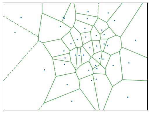
To keep the code effective, we renounce calculating the Voronoi tessellation for each partition of the road network. Instead, tessellate the whole road network once using roads and calculate the population and area of each road cell. Then, we can use this information to determine the population density of each Superblock repeatedly. More on the edge tesselation in the previous chapter Street Tessellation.

There are two approaches we want to consider integrating the population raster data over the road cells. The first approach is to use up-sampled raster data, as we did before. The second approach is to polygonize the raster data and intersect the road cells with it. For both, we need to consider used memory and computation time. Loading in a big city with an up-sampled raster dataset can take a lot of time and memory, but it needs to be up-sampled to reach better population approximations. Calculating intersections between polygons could be computationally heavy.

Data Preparation

First, let’s get an example road network and tessellate it. We are Using La Crosse, Wisconsin as an example. By the Native American Neshnabé/Potawatomi, it is called ensewaksak. The working CRS is the World Mollweide projection, as it is an equal-area projection, and the GHS-POP raster data is in this projection. But the edge cells need to be calculated in the local CRS, to avoid distortion.

lc_graph = ox.graph_from_place("La Crosse, La Crosse County, Wisconsin, United "
                                 "States",
                            network_type="drive")
lc_graph = ox.project_graph(lc_graph)  # to local UTM zone
# Get Road Cells
lc_road_cells = get_edge_cells(lc_graph)
# Project to World Mollweide
lc_road_cells = lc_road_cells.to_crs("World Mollweide")

2024-09-21 05:45:15,974 |     INFO | tessellation.py:101 | Calculating edge cells for graph with 4799 edges.

2024-09-21 05:45:21,915 |     INFO | tessellation.py:155 | Tessellated 2606 edge cells in 0:00:05.

How does the tessellation look like?

# random color of CSS4_COLORS
lc_road_cells["color_name"] = np.random.choice(list(CSS4_COLORS.keys()),
                                               size=len(lc_road_cells))
lc_road_cells.explore(color="color_name", style_kwds={"color": "black", "opacity": 0.5,
                                                      "weight": 1}, zoom_start=14)

Make this Notebook Trusted to load map: File -> Trust Notebook

We need to get the GHS-POP raster data for the area of interest. For that we can use the get_ghsl function from the superblockify package. It needs a bounding box of the whole are in Mollweide projection, and it will download the raster data and return the file path(s) to the raster data. The raster data is in GeoTIFF format. For that, we take the union of all road cells and get the bounding box of it. When looking at the union, the skewness of our projection is visible.

lc_road_cells.unary_union

lc_bbox = lc_road_cells.unary_union.bounds
lc_ghsl = get_ghsl(lc_bbox)

2024-09-21 05:45:24,879 |     INFO | ghsl.py:129 | Using the GHSL raster tiles for the bounding box (-7466813.851098051, 5203806.91829774, -7458948.00461384, 5217156.191940161).

Up-sampled Raster Data

Try to load the raster data inside the bounding box into memory and scale up by a factor of 10. The original cells are 100m x 100m, so the up-sampled cells are 10m x 10m. For that, we use the resample_load_window function from the superblockify package.

lc_ghsl_upsampled, lc_affine_upsampled = resample_load_window(
    file=lc_ghsl, resample_factor=10, window=lc_road_cells)
lc_ghsl_upsampled /= 10 ** 2

The resampling strategy for upscaling is nearest, so to conserve the population values, we needed to divide the population values by the resample factor squared.

Now, we can use the zonal_stats function from the rasterstats package to calculate the population and area of each road cell. Just like we did in the Population Density notebook.

lc_zonal_stats = zonal_stats(lc_road_cells, lc_ghsl_upsampled,
                             affine=lc_affine_upsampled,
                             stats=["sum"], nodata=0, all_touched=False)
lc_zonal_stats

Show code cell output Hide code cell output

[{'sum': 27.736934700012206},
 {'sum': 57.325349143743516},
 {'sum': 9.597237935066223},
 {'sum': 85.20203415870667},
 {'sum': 42.575706710815425},
 {'sum': 78.53595002174377},
 {'sum': 13.251874021291734},
 {'sum': None},
 {'sum': 0.399763503074646},
 {'sum': 1.403202327596955},
 {'sum': 10.477114752978085},
 {'sum': None},
 {'sum': None},
 {'sum': 0.02859644591808319},
 {'sum': 0.0067599741369485855},
 {'sum': None},
 {'sum': 9.21284694671631},
 {'sum': 9.986630411148072},
 {'sum': 7.182888542711735},
 {'sum': 6.0987732481956485},
 {'sum': 2.4471438860893246},
 {'sum': None},
 {'sum': 9.988775436878203},
 {'sum': 0.22754573822021484},
 {'sum': 11.274066665172576},
 {'sum': 2.8637148094177247},
 {'sum': 27.51528042136226},
 {'sum': 7.271112310886382},
 {'sum': 21.28383520126343},
 {'sum': 1.1894436836242677},
 {'sum': 11.531901578903199},
 {'sum': 32.476610288619995},
 {'sum': 25.381733250617977},
 {'sum': 3.612999219894409},
 {'sum': 14.5295338344574},
 {'sum': 5.6516998624801635},
 {'sum': 19.610420441627504},
 {'sum': 8.863997044563293},
 {'sum': None},
 {'sum': 1.551448173522949},
 {'sum': 14.391211013793944},
 {'sum': 45.61249006152153},
 {'sum': 8.7447283744812},
 {'sum': 10.783017654418945},
 {'sum': 12.062019405364989},
 {'sum': 9.158895301818847},
 {'sum': 0.20598119735717774},
 {'sum': 10.314951210021974},
 {'sum': 34.8305658531189},
 {'sum': 91.87395264625549},
 {'sum': None},
 {'sum': 1.3563079482316969},
 {'sum': 13.912750692367553},
 {'sum': 38.57099239945411},
 {'sum': 0.5920436096191406},
 {'sum': 3.6333688962459565},
 {'sum': 43.77681309700013},
 {'sum': 7.527082061767579},
 {'sum': 0.8349046707153321},
 {'sum': 15.528937244415284},
 {'sum': 5.709406366348267},
 {'sum': 15.903507251739502},
 {'sum': 10.918051490783691},
 {'sum': 10.939556102752684},
 {'sum': 23.394271221160892},
 {'sum': 45.4419010257721},
 {'sum': 20.10714277267456},
 {'sum': 19.34319558620453},
 {'sum': 8.774801943302155},
 {'sum': 12.061386775970458},
 {'sum': 21.05259316921234},
 {'sum': 3.7521368980407717},
 {'sum': 16.279863834381104},
 {'sum': 64.8140503692627},
 {'sum': 16.183352165222168},
 {'sum': 13.339902992248534},
 {'sum': 24.879065704345706},
 {'sum': 23.279370880126955},
 {'sum': 22.20684398651123},
 {'sum': 31.50952657699585},
 {'sum': 24.053794536590573},
 {'sum': 15.686120090484618},
 {'sum': 5.565841751098633},
 {'sum': 48.530771341323856},
 {'sum': 6.880045995712281},
 {'sum': 2.6899125576019287},
 {'sum': 9.902365531921387},
 {'sum': 9.282640342712401},
 {'sum': 52.973795909881595},
 {'sum': 7.584374923706056},
 {'sum': 39.34828866958618},
 {'sum': 8.760193309783935},
 {'sum': 16.332075920104984},
 {'sum': 16.637885570526123},
 {'sum': 20.819307518005374},
 {'sum': 18.965822286605835},
 {'sum': 11.54761604309082},
 {'sum': 10.142733743190766},
 {'sum': 22.913720169067382},
 {'sum': 18.935145053863526},
 {'sum': 49.21882862091065},
 {'sum': 15.026035881042482},
 {'sum': 7.775572395324707},
 {'sum': 3.0718676376342775},
 {'sum': 17.684419555664064},
 {'sum': 10.66260931968689},
 {'sum': 12.560982036590577},
 {'sum': 5.079501571655274},
 {'sum': 4.45970395565033},
 {'sum': 0.23600312709808347},
 {'sum': 2.8699823474884036},
 {'sum': 10.683334627151492},
 {'sum': 23.554101734161378},
 {'sum': 38.01632788181305},
 {'sum': 5.861234016418457},
 {'sum': 23.60091625213623},
 {'sum': 32.360697984695435},
 {'sum': 7.080295095443725},
 {'sum': 33.598302860260006},
 {'sum': 30.821837368011472},
 {'sum': 2.460548038482666},
 {'sum': 22.706986932754514},
 {'sum': 25.982524309158325},
 {'sum': 0.704912371635437},
 {'sum': 16.021509915590286},
 {'sum': 2.311175537109375},
 {'sum': 12.759120368957518},
 {'sum': 9.346754379272461},
 {'sum': 9.60316795349121},
 {'sum': 17.334847927093506},
 {'sum': 37.88636428833008},
 {'sum': 31.22610486984253},
 {'sum': 19.869698429107665},
 {'sum': 54.00243092536927},
 {'sum': 33.31645170211792},
 {'sum': 16.28328014373779},
 {'sum': 16.899838542938234},
 {'sum': 21.86838144302368},
 {'sum': 8.42118396759033},
 {'sum': 27.61464000701904},
 {'sum': 9.973985934257508},
 {'sum': 8.661177988052367},
 {'sum': 5.259655017852783},
 {'sum': 22.599429359436034},
 {'sum': 0.7764247369766235},
 {'sum': 4.122556605339049},
 {'sum': 5.929441874027251},
 {'sum': 0.13979608297348023},
 {'sum': 0.8673437285423279},
 {'sum': 4.715267920494079},
 {'sum': 4.249354844093323},
 {'sum': 8.807896604537964},
 {'sum': 12.332220578193667},
 {'sum': 19.997155360877514},
 {'sum': 3.9926023623347278},
 {'sum': 9.218991367816924},
 {'sum': 13.809043159484862},
 {'sum': 2.8045876121521},
 {'sum': 0.2749660083651543},
 {'sum': 0.9428110167384147},
 {'sum': 2.105606622695923},
 {'sum': 0.08274391174316406},
 {'sum': 0.16548782348632812},
 {'sum': 5.46232493877411},
 {'sum': 7.614660153388977},
 {'sum': 7.246677436828613},
 {'sum': 0.006882149577140808},
 {'sum': 0.4245280910283328},
 {'sum': 1.9565142267942428},
 {'sum': 11.871370921134949},
 {'sum': 1.443102343082428},
 {'sum': 19.420064611434935},
 {'sum': 19.913752937316897},
 {'sum': 4.726371240615845},
 {'sum': 5.178878297805786},
 {'sum': 98.95620507240295},
 {'sum': 38.88503512382507},
 {'sum': 3.621687088012696},
 {'sum': 21.551640833616254},
 {'sum': 30.241707029938695},
 {'sum': 0.6332982254028321},
 {'sum': 0.7472045135498047},
 {'sum': 10.90181888103485},
 {'sum': 9.672452557086944},
 {'sum': 15.889475452899932},
 {'sum': 12.845588750839234},
 {'sum': 57.76188638061285},
 {'sum': 34.38131134033203},
 {'sum': 38.20441918849945},
 {'sum': 24.298406295776367},
 {'sum': 46.467518463134766},
 {'sum': 57.37507019042968},
 {'sum': 30.223601744174957},
 {'sum': 35.86291999816895},
 {'sum': 52.56343090057373},
 {'sum': 2.804838562011719},
 {'sum': 12.776551389694214},
 {'sum': 30.355435018539428},
 {'sum': 43.522705039978035},
 {'sum': 23.04573190689087},
 {'sum': 11.06228972196579},
 {'sum': 74.94886870697141},
 {'sum': 31.175020027160645},
 {'sum': 9.277140502929687},
 {'sum': 1.496576220393181},
 {'sum': 136.8211680650711},
 {'sum': 5.2869447898864745},
 {'sum': 10.748219432830812},
 {'sum': 2.741246604919434},
 {'sum': 29.57303462982178},
 {'sum': 11.221705341339112},
 {'sum': 90.26561373233795},
 {'sum': 1.0008994483947753},
 {'sum': 3.3895029067993168},
 {'sum': 57.36833569526672},
 {'sum': 0.6703520011901856},
 {'sum': 4.922669099569321},
 {'sum': 0.10272883415222168},
 {'sum': 9.954598378241062},
 {'sum': 37.13566722869873},
 {'sum': 19.823162078857422},
 {'sum': 27.506619949340823},
 {'sum': 4.138906545042991},
 {'sum': 4.634250955581665},
 {'sum': 10.693077182769775},
 {'sum': 34.29150991678238},
 {'sum': 0.9661161416769026},
 {'sum': 3.6138537216186526},
 {'sum': 7.853363027572632},
 {'sum': 35.903636322021484},
 {'sum': 49.21193687438964},
 {'sum': 1.0163430404663085},
 {'sum': 0.18440183456987144},
 {'sum': 0.024690250456333163},
 {'sum': 0.006690916940569877},
 {'sum': 1.1136795899271967},
 {'sum': 0.7125074034929277},
 {'sum': 0.10296257555484772},
 {'sum': 8.964328391551971},
 {'sum': 82.29395275115967},
 {'sum': 30.755844078063966},
 {'sum': 29.87458963394165},
 {'sum': 38.64514499664307},
 {'sum': 1.5189695739746094},
 {'sum': 0.18987119674682618},
 {'sum': 0.5142012405395509},
 {'sum': 0.3243300437927246},
 {'sum': 20.72265501022339},
 {'sum': 14.124819335937499},
 {'sum': 7.006377563476562},
 {'sum': 7.638710556030274},
 {'sum': 47.830800247192386},
 {'sum': 27.300691909790043},
 {'sum': 25.90570213317871},
 {'sum': 61.126611900329586},
 {'sum': 75.2969554901123},
 {'sum': 32.37028007507324},
 {'sum': 8.729962368011474},
 {'sum': 12.775760383605958},
 {'sum': 15.97017195701599},
 {'sum': 22.500070800781252},
 {'sum': 12.727870979309083},
 {'sum': 10.62649179458618},
 {'sum': 33.45295812606811},
 {'sum': 15.843661403656007},
 {'sum': 35.06832845687866},
 {'sum': 49.126378388404845},
 {'sum': 15.028181018829345},
 {'sum': 64.1684658241272},
 {'sum': 12.000565648078918},
 {'sum': 33.287354469299316},
 {'sum': 41.63470988273621},
 {'sum': 13.668164339065552},
 {'sum': 23.740465202331542},
 {'sum': 20.4936411857605},
 {'sum': 26.02949520111084},
 {'sum': 12.0363734126091},
 {'sum': 10.015463523864746},
 {'sum': 12.007115497589112},
 {'sum': 17.395006003379823},
 {'sum': 19.31197748184204},
 {'sum': 8.943642082214357},
 {'sum': 12.528310222625732},
 {'sum': 26.80551664352417},
 {'sum': 21.89610563278198},
 {'sum': 22.671456842422486},
 {'sum': 9.108699502944948},
 {'sum': 19.442693760395052},
 {'sum': 2.3505996465682983},
 {'sum': 1.9061580276489258},
 {'sum': 0.7446951293945312},
 {'sum': 1.3032164764404297},
 {'sum': 6.454024538993835},
 {'sum': 14.759866418838502},
 {'sum': 9.674940028190614},
 {'sum': 85.12165424346924},
 {'sum': 20.953614192008974},
 {'sum': 17.653895893096923},
 {'sum': 18.603180713653565},
 {'sum': 25.85831932067871},
 {'sum': 51.70731159210206},
 {'sum': 17.431900005340577},
 {'sum': 13.83742826461792},
 {'sum': 41.80303977012635},
 {'sum': 17.061766147613525},
 {'sum': 6.588129024505615},
 {'sum': 16.378577251434326},
 {'sum': 14.635418739318848},
 {'sum': 14.091799736022947},
 {'sum': 26.014918212890628},
 {'sum': 12.309328575134277},
 {'sum': 23.066308097839354},
 {'sum': 25.044627857208255},
 {'sum': 14.34100595474243},
 {'sum': 18.894955310821533},
 {'sum': 11.84447925567627},
 {'sum': 5.55043737411499},
 {'sum': 8.989890155792237},
 {'sum': 1.0860137557983398},
 {'sum': 5.099041957855224},
 {'sum': 17.354841499328614},
 {'sum': 9.542497062683106},
 {'sum': 63.09284478187561},
 {'sum': 11.763956050872803},
 {'sum': 101.48530504703521},
 {'sum': 73.46337113380432},
 {'sum': 0.7362484005093575},
 {'sum': 5.6842017841339105},
 {'sum': 12.866775379180908},
 {'sum': 10.462252006530761},
 {'sum': 11.047516155242919},
 {'sum': 48.68734745025634},
 {'sum': 4.074535366296768},
 {'sum': 2.6597952926158905},
 {'sum': 0.05622429072856903},
 {'sum': 11.987523040771483},
 {'sum': 9.08901505947113},
 {'sum': 6.081677074432373},
 {'sum': 15.659283866882324},
 {'sum': 15.194161987304685},
 {'sum': 33.25270669937134},
 {'sum': 14.22840633392334},
 {'sum': 15.317574405670165},
 {'sum': 16.352264099121093},
 {'sum': 47.08630155563354},
 {'sum': 15.347532768249515},
 {'sum': 15.814155464172362},
 {'sum': 40.37996850967408},
 {'sum': 13.172424888610841},
 {'sum': 15.814924926757813},
 {'sum': 16.911363105773923},
 {'sum': 12.771377048492429},
 {'sum': 15.377923984527587},
 {'sum': 15.297279605865477},
 {'sum': 12.48398675918579},
 {'sum': 17.883025913238527},
 {'sum': 14.755050773620605},
 {'sum': 13.218338737487791},
 {'sum': 14.9899645614624},
 {'sum': 9.763033571243286},
 {'sum': 9.43280506134033},
 {'sum': 8.366717376708984},
 {'sum': 8.440858869552612},
 {'sum': 11.212102966308596},
 {'sum': 79.35457859039306},
 {'sum': 48.46744565963745},
 {'sum': 10.444705867767336},
 {'sum': 16.98435874938965},
 {'sum': 5.967904205322266},
 {'sum': 9.887896919250489},
 {'sum': 4.1578811931610105},
 {'sum': 9.867211017608643},
 {'sum': 5.635001697540284},
 {'sum': 3.1497114944458007},
 {'sum': 15.159847068786622},
 {'sum': 18.14793712615967},
 {'sum': 0.5171493911743164},
 {'sum': 0.86918776512146},
 {'sum': 0.4905795860290527},
 {'sum': 43.963076844215394},
 {'sum': 25.550788230895996},
 {'sum': 3.373516082763672},
 {'sum': 8.737983570098876},
 {'sum': 24.961077938079832},
 {'sum': 14.713462867736817},
 {'sum': 9.056583423614502},
 {'sum': 18.47494993209839},
 {'sum': 8.146451530456542},
 {'sum': 47.79129108428955},
 {'sum': 12.79135353088379},
 {'sum': 10.522689046859742},
 {'sum': 9.433854084014893},
 {'sum': 2.1725437927246087},
 {'sum': 2.598998394012451},
 {'sum': 17.291949310302734},
 {'sum': 70.52204416275025},
 {'sum': 10.243543567657472},
 {'sum': 1.4403462553024293},
 {'sum': 19.502734394073485},
 {'sum': 29.456876831054686},
 {'sum': 15.3178303527832},
 {'sum': 14.901261653900146},
 {'sum': 46.555399360656736},
 {'sum': 15.341924991607666},
 {'sum': 15.321520957946777},
 {'sum': 42.99302259445191},
 {'sum': 23.321945724487303},
 {'sum': 24.13576286315918},
 {'sum': 20.02904552459717},
 {'sum': 37.42528448104859},
 {'sum': 19.936909351348874},
 {'sum': 18.57600696563721},
 {'sum': 44.987581834793104},
 {'sum': 16.382890510559083},
 {'sum': 17.4077038192749},
 {'sum': 20.09637660980225},
 {'sum': 28.122585598230362},
 {'sum': 12.513875083923338},
 {'sum': 12.56921401977539},
 {'sum': 8.961044883728027},
 {'sum': 12.650244998931885},
 {'sum': 15.864584188461304},
 {'sum': 1.3410041534900665},
 {'sum': 0.16548784255981444},
 {'sum': 8.470907592773438},
 {'sum': 14.925606656074525},
 {'sum': 11.862726736068726},
 {'sum': 27.316270465850828},
 {'sum': 9.119097433090209},
 {'sum': 53.62132207870483},
 {'sum': 11.747446193695069},
 {'sum': 13.205208492279052},
 {'sum': 19.463404636383057},
 {'sum': 19.143651428222654},
 {'sum': 15.71608983039856},
 {'sum': 16.473800945281983},
 {'sum': 63.65574956893921},
 {'sum': 15.752713775634767},
 {'sum': 21.072506313323977},
 {'sum': 29.307043018341062},
 {'sum': 35.83940008163452},
 {'sum': 41.45595817565918},
 {'sum': 26.35171981811523},
 {'sum': 32.3945546913147},
 {'sum': 43.26556869506835},
 {'sum': 10.159970760345459},
 {'sum': 18.681372470855713},
 {'sum': 11.23190855026245},
 {'sum': 30.130626430511477},
 {'sum': 33.500787506103514},
 {'sum': 30.267813224792484},
 {'sum': 21.151561126708984},
 {'sum': 31.39238775253296},
 {'sum': 11.896669120788577},
 {'sum': 26.563177375793458},
 {'sum': 17.603765869140624},
 {'sum': 11.310605182647706},
 {'sum': 15.047473526000976},
 {'sum': 13.751632022857665},
 {'sum': 17.545648946762086},
 {'sum': 14.892851905822752},
 {'sum': 7.050197410583495},
 {'sum': 32.822062335014344},
 {'sum': 7.008846721649169},
 {'sum': 37.84215038868598},
 {'sum': 23.175568451881404},
 {'sum': 6.608662478923797},
 {'sum': 11.680714678764343},
 {'sum': 55.643736085891724},
 {'sum': 18.393563270568848},
 {'sum': 0.7736093044281005},
 {'sum': 32.40539176940918},
 {'sum': 6.645176548957826},
 {'sum': 4.700140647888183},
 {'sum': 7.432553634643555},
 {'sum': 3.4615586280822757},
 {'sum': 10.248969812393188},
 {'sum': 27.059111404418942},
 {'sum': 7.033830947875976},
 {'sum': 13.860751876831053},
 {'sum': 9.452105522155762},
 {'sum': 28.6788911819458},
 {'sum': 10.698963012695312},
 {'sum': 51.45630096912383},
 {'sum': 23.600359497070315},
 {'sum': 44.96813637733459},
 {'sum': 22.722966456413268},
 {'sum': 19.90240612030029},
 {'sum': 61.80304237365723},
 {'sum': 11.43451085090637},
 {'sum': 14.052908363342286},
 {'sum': 8.266985092163086},
 {'sum': 31.091964111328124},
 {'sum': 23.726217675209046},
 {'sum': 13.569327774047853},
 {'sum': 13.060551519393922},
 {'sum': 26.541215019226076},
 {'sum': 7.9946593761444085},
 {'sum': 48.03370130538941},
 {'sum': 27.76058055877686},
 {'sum': 18.944811477661133},
 {'sum': 14.341558761596678},
 {'sum': 12.287614459991454},
 {'sum': 86.98383458256721},
 {'sum': 42.881294505745174},
 {'sum': 82.15176138877868},
 {'sum': 48.01412265777588},
 {'sum': 48.01412265777588},
 {'sum': 7.218820877075196},
 {'sum': 36.49451505184173},
 {'sum': 6.548099460601808},
 {'sum': 26.061658992767335},
 {'sum': 19.928680915832523},
 {'sum': 8.779589805603027},
 {'sum': 25.211387634277344},
 {'sum': 26.16627941131592},
 {'sum': 151.44076132297516},
 {'sum': 23.203449401855465},
 {'sum': 14.232903919219973},
 {'sum': 14.572143733501436},
 {'sum': 12.146479101181031},
 {'sum': 39.53089958190918},
 {'sum': 50.5726021194458},
 {'sum': 102.44660257339478},
 {'sum': 50.28578632354736},
 {'sum': 42.353961334228515},
 {'sum': 46.4917317199707},
 {'sum': 17.998053607940676},
 {'sum': 23.58274766921997},
 {'sum': 16.23229139328003},
 {'sum': 20.165146889686582},
 {'sum': 19.077402973175047},
 {'sum': 22.254235649108885},
 {'sum': 74.23831029891969},
 {'sum': 15.736655168533325},
 {'sum': 22.331369514465333},
 {'sum': 26.32501848220825},
 {'sum': 50.641179199218755},
 {'sum': 52.29387310028076},
 {'sum': 17.376220321655275},
 {'sum': 21.151136512756345},
 {'sum': 23.995732498168945},
 {'sum': 68.30814250946045},
 {'sum': 29.549917449951174},
 {'sum': 45.07474262237548},
 {'sum': 22.076403541564936},
 {'sum': 17.040777339935307},
 {'sum': 1.1444770431518554},
 {'sum': 4.261636872291565},
 {'sum': 14.17936388015747},
 {'sum': 2.980304646492004},
 {'sum': 15.212382221221922},
 {'sum': 15.230544776916503},
 {'sum': 18.709451274871824},
 {'sum': 37.77533836364746},
 {'sum': 26.07488346099853},
 {'sum': 39.67199878692627},
 {'sum': 27.910703926086427},
 {'sum': 21.43903982162476},
 {'sum': 1.1827083587646483},
 {'sum': 7.492833786010742},
 {'sum': 34.165265274047854},
 {'sum': 25.873409500122072},
 {'sum': 25.418934612274168},
 {'sum': 23.132096099853513},
 {'sum': 29.475353641510008},
 {'sum': 14.624572315216064},
 {'sum': 13.648854179382324},
 {'sum': 10.808578643798828},
 {'sum': 13.604961767196656},
 {'sum': 10.200377111434936},
 {'sum': 15.544131460189817},
 {'sum': 16.119558315277096},
 {'sum': 25.522212352752682},
 {'sum': 9.041732282638549},
 {'sum': 10.055219869613648},
 {'sum': 57.3100475692749},
 {'sum': 0.5809731674194336},
 {'sum': 3.9580772304534912},
 {'sum': 13.556724739074706},
 {'sum': 1.3555014896392823},
 {'sum': 21.602500772476194},
 {'sum': 29.71934661865234},
 {'sum': 16.00473222732544},
 {'sum': 9.921388549804687},
 {'sum': 2.4964186859130857},
 {'sum': 53.843078022003176},
 {'sum': 1.0796439361572265},
 {'sum': 50.69131660461426},
 {'sum': 10.697833442687989},
 {'sum': 11.187334022521974},
 {'sum': 15.283116054534911},
 {'sum': 14.815284366607667},
 {'sum': 11.228231830596922},
 {'sum': 11.532300701141356},
 {'sum': 1.7335149681568145},
 {'sum': 7.393299465179442},
 {'sum': 19.891060771942136},
 {'sum': 70.86284770965577},
 {'sum': 14.369502849578856},
 {'sum': 13.232961444854736},
 {'sum': 23.86110065460205},
 {'sum': 14.634822921752932},
 {'sum': 22.08687042236328},
 {'sum': None},
 {'sum': 45.86883251190186},
 {'sum': 11.331518630981446},
 {'sum': 3.7951988875865936},
 {'sum': 11.910753631591795},
 {'sum': 31.597267608642582},
 {'sum': 47.90765981197357},
 {'sum': 45.160299453735355},
 {'sum': 15.50386313736439},
 {'sum': 28.827352684736255},
 {'sum': 39.04673884868622},
 {'sum': 26.922058191299442},
 {'sum': 44.09754425048828},
 {'sum': 40.22713363647461},
 {'sum': 37.11064046859741},
 {'sum': 0.5346172404289247},
 {'sum': 7.334097948074342},
 {'sum': 4.039052460193634},
 {'sum': 12.301512832641603},
 {'sum': 11.520285015106202},
 {'sum': 16.604218454360964},
 {'sum': 13.610353374481202},
 {'sum': 14.240515022277833},
 {'sum': 15.220611133575442},
 {'sum': 30.72229145050049},
 {'sum': 16.366435127258303},
 {'sum': 28.3581494140625},
 {'sum': 18.99946304321289},
 {'sum': 16.508916416168212},
 {'sum': 19.024236278533934},
 {'sum': 29.680274658203125},
 {'sum': 4.369757385253907},
 {'sum': 32.60094951629638},
 {'sum': 16.363222913742064},
 {'sum': 14.370696547031404},
 {'sum': 20.301868779659273},
 {'sum': 10.990688705444335},
 {'sum': 15.789670848846434},
 {'sum': 13.437755799293518},
 {'sum': 6.101349711418151},
 {'sum': 11.592327919006346},
 {'sum': 19.755012941360476},
 {'sum': 24.8639946937561},
 {'sum': 16.564805698394775},
 {'sum': 17.77118263244629},
 {'sum': 22.36512773513794},
 {'sum': 22.625250072479247},
 {'sum': 23.097777099609374},
 {'sum': 6.4510803794860845},
 {'sum': 53.55474775314331},
 {'sum': 43.347017707824705},
 {'sum': 101.23717079162597},
 {'sum': 15.781080551147461},
 {'sum': 17.428926639556884},
 {'sum': 78.47873725891112},
 {'sum': 30.323897094726565},
 {'sum': 18.295516452789307},
 {'sum': 295.3136851501465},
 {'sum': 9.718619017601014},
 {'sum': 13.331508173942566},
 {'sum': 7.854272341728212},
 {'sum': 38.42088615417481},
 {'sum': 15.965241737365723},
 {'sum': 22.071937255859375},
 {'sum': 33.05832344055176},
 {'sum': 34.02538317680359},
 {'sum': 25.77500633239746},
 {'sum': 6.092020106315612},
 {'sum': 1.8312551498413083},
 {'sum': 5.838563880920411},
 {'sum': 58.224616832137116},
 {'sum': 34.34661476135254},
 {'sum': 22.15588893890381},
 {'sum': 27.084772605895992},
 {'sum': 3.0487042903900146},
 {'sum': 51.70077691078186},
 {'sum': 3.057378010749817},
 {'sum': 8.191182632446289},
 {'sum': 14.333359279632568},
 {'sum': 13.336913032531736},
 {'sum': 35.384829177856446},
 {'sum': 12.382957515716551},
 {'sum': 30.76994255065918},
 {'sum': 16.734730458259584},
 {'sum': 0.09927147656679154},
 {'sum': 6.599063566476106},
 {'sum': 28.77404449537397},
 {'sum': 3.517550600767135},
 {'sum': 19.297422440350054},
 {'sum': 2.8196396258473397},
 {'sum': 7.912085141837597},
 {'sum': 4.358126411437988},
 {'sum': 30.190073717832565},
 {'sum': 17.64660457611084},
 {'sum': 13.605199737548826},
 {'sum': 30.941535110473634},
 {'sum': 28.778232898712158},
 {'sum': 3.113239479064941},
 {'sum': 24.26699550628662},
 {'sum': 14.78092933654785},
 {'sum': 22.712428741455078},
 {'sum': 11.909948892593384},
 {'sum': 12.738376178741454},
 {'sum': 39.89640069961547},
 {'sum': 25.816679344177242},
 {'sum': 35.24737482905388},
 {'sum': 18.413220291137694},
 {'sum': 45.22750051498413},
 {'sum': 18.6248370552063},
 {'sum': 27.667921714782715},
 {'sum': 87.1382149887085},
 {'sum': 25.19826271057129},
 {'sum': 28.704687652587893},
 {'sum': 121.35065307617187},
 {'sum': 110.43622665405275},
 {'sum': 137.13997734069824},
 {'sum': 29.703600006103514},
 {'sum': 209.9201789665222},
 {'sum': 7.870704946517944},
 {'sum': 2.7252999114990235},
 {'sum': 1.7881571102142335},
 {'sum': 37.50104650497437},
 {'sum': 15.848726329803466},
 {'sum': 22.33993811607361},
 {'sum': 12.2316494846344},
 {'sum': 10.38101390838623},
 {'sum': 9.960908188819884},
 {'sum': 18.963027420043943},
 {'sum': 1.466886730194092},
 {'sum': 50.31673023223877},
 {'sum': 76.22944072723388},
 {'sum': 22.05133045196533},
 {'sum': 16.029520130157472},
 {'sum': 12.20405295372009},
 {'sum': 11.248738861083986},
 {'sum': 7.5198991298675555},
 {'sum': 33.26730326652527},
 {'sum': 10.782324390411375},
 {'sum': 27.561724987030033},
 {'sum': 10.926154842376707},
 {'sum': 8.04711380004883},
 {'sum': 0.6119281196594238},
 {'sum': 17.19037231445312},
 {'sum': 14.147854862213133},
 {'sum': 38.31215330123901},
 {'sum': 20.21529598236084},
 {'sum': 14.11817928314209},
 {'sum': 15.529999408721924},
 {'sum': 12.119538989067076},
 {'sum': 0.024819934368133546},
 {'sum': 4.887043580710888},
 {'sum': None},
 {'sum': None},
 {'sum': 2.9829302644729614},
 {'sum': 8.958555026054384},
 {'sum': 4.77674315929413},
 {'sum': 25.16581190109253},
 {'sum': 26.25877248764038},
 {'sum': 9.999871311187743},
 {'sum': 21.507296562194824},
 {'sum': 15.10082953453064},
 {'sum': 8.035700092315674},
 {'sum': 19.088291225433352},
 {'sum': 42.78639928817749},
 {'sum': 18.731200571060178},
 {'sum': 17.389673500061036},
 {'sum': 36.043468379974364},
 {'sum': 25.36994623184204},
 {'sum': 19.78300256729126},
 {'sum': 21.552526626586918},
 {'sum': 49.18373365402221},
 {'sum': 19.863356781005862},
 {'sum': 27.070535736083986},
 {'sum': 39.29863079071045},
 {'sum': 49.818943195343024},
 {'sum': 9.40803508758545},
 {'sum': 14.775067043304444},
 {'sum': 15.953770980834959},
 {'sum': 28.72752416610718},
 {'sum': 14.444765319824219},
 {'sum': 15.295666675567627},
 {'sum': 25.568113861083983},
 {'sum': 39.681825733184816},
 {'sum': 30.139467773437502},
 {'sum': 17.013571701049806},
 {'sum': 25.758639221191405},
 {'sum': 36.40283081054688},
 {'sum': 37.75793830871582},
 {'sum': 23.202285270690922},
 {'sum': 26.666582183837892},
 {'sum': 16.441084070205687},
 {'sum': 13.957937488555906},
 {'sum': 19.946139297485352},
 {'sum': 83.16860460281373},
 {'sum': 17.156447038650516},
 {'sum': 7.651460270881652},
 {'sum': 26.155818510055546},
 {'sum': 81.10375291824342},
 {'sum': 43.59011306762695},
 {'sum': 10.653226943016051},
 {'sum': 16.359948596954347},
 {'sum': 10.764034814834595},
 {'sum': 13.340300550460814},
 {'sum': 3.038818626403808},
 {'sum': 10.84472261428833},
 {'sum': 3.277177734375},
 {'sum': 4.03452657699585},
 {'sum': 10.149247131347657},
 {'sum': 11.307531127929687},
 {'sum': 22.963079833984374},
 {'sum': 30.40385459899902},
 {'sum': 48.87960012435913},
 {'sum': 11.37206665992737},
 {'sum': 18.531636800765995},
 {'sum': 29.954289870262148},
 {'sum': 21.18126865386963},
 {'sum': 17.583240566253664},
 {'sum': 30.9683193397522},
 {'sum': 35.7480014038086},
 {'sum': 23.678406620025633},
 {'sum': 11.224072608947754},
 {'sum': 2.0676580238342286},
 {'sum': 0.17419086456298827},
 {'sum': 93.12916111469268},
 {'sum': 7.611734352111817},
 {'sum': 1.918353862762451},
 {'sum': 10.560236549377441},
 {'sum': 27.301256675720214},
 {'sum': 36.688502883911134},
 {'sum': 14.65131362915039},
 {'sum': 11.12120527267456},
 {'sum': 24.381989431381225},
 {'sum': 10.893086433410645},
 {'sum': 10.334357566833496},
 {'sum': 17.404937715530394},
 {'sum': 22.514844312667847},
 {'sum': 8.890370769500734},
 {'sum': 12.162730712890625},
 {'sum': 13.23465829849243},
 {'sum': 25.732678813934324},
 {'sum': 30.947960376739502},
 {'sum': 30.533884563446037},
 {'sum': 21.795296516418457},
 {'sum': 23.175834674835208},
 {'sum': 2.020016059875488},
 {'sum': 23.804464244842528},
 {'sum': 14.357351589202882},
 {'sum': 51.78753074645996},
 {'sum': 5.769486446380615},
 {'sum': 37.642355327606204},
 {'sum': 9.052960934638977},
 {'sum': 32.224383192062376},
 {'sum': 9.472807359695434},
 {'sum': 6.296509456634521},
 {'sum': 10.309912767410278},
 {'sum': 14.340286645889282},
 {'sum': 7.065372667312622},
 {'sum': 14.92251763343811},
 {'sum': 20.78350803375244},
 {'sum': 0.25487810134887695},
 {'sum': 32.42156339645386},
 {'sum': 18.3456125831604},
 {'sum': 16.026280059814454},
 {'sum': 5.282147941589356},
 {'sum': 7.326283988952636},
 {'sum': 7.641970367431641},
 {'sum': 16.24883243560791},
 {'sum': 52.666372013092044},
 {'sum': 5.886952590942382},
 {'sum': 9.64273190021515},
 {'sum': 0.9667221832275392},
 {'sum': 18.142445230484007},
 {'sum': 25.033783435821533},
 {'sum': 35.529874114990236},
 {'sum': 22.692517013549804},
 {'sum': 34.361020698547364},
 {'sum': 16.26845283508301},
 {'sum': 12.283345851898194},
 {'sum': 41.27593231201172},
 {'sum': 17.245030212402344},
 {'sum': 16.99594648361206},
 {'sum': 14.532542190551759},
 {'sum': 31.395512447357177},
 {'sum': 50.761097240448},
 {'sum': 29.74905040740967},
 {'sum': 0.2440147590637207},
 {'sum': 8.035041637420655},
 {'sum': 12.457240920066836},
 {'sum': 39.74749008491635},
 {'sum': 12.392866706848146},
 {'sum': 22.88823221564293},
 {'sum': 11.174190645217895},
 {'sum': 36.32022419929505},
 {'sum': 73.23920006752014},
 {'sum': 15.237160739898682},
 {'sum': 27.198902378082277},
 {'sum': 39.86389284133911},
 {'sum': 11.309413871765138},
 {'sum': 25.25816873550415},
 {'sum': 22.645623512268063},
 {'sum': 20.293909845352175},
 {'sum': 2.4884135913848877},
 {'sum': 25.644057388305665},
 {'sum': 28.58958445549011},
 {'sum': 16.856267652511598},
 {'sum': 45.855820922851564},
 {'sum': 34.11645612716674},
 {'sum': 69.29390159606933},
 {'sum': 10.60279185295105},
 {'sum': 63.823746032714844},
 {'sum': 60.7598101425171},
 {'sum': 18.299052200317384},
 {'sum': 112.8685647201538},
 {'sum': 23.49467529296875},
 {'sum': 24.040220661163332},
 {'sum': 8.064394686222077},
 {'sum': 154.76840766906741},
 {'sum': 321.36337673187256},
 {'sum': 16.433403460383413},
 {'sum': 7.907710304260254},
 {'sum': 7.9020426559448245},
 {'sum': 25.133461284637455},
 {'sum': 4.4855666351318355},
 {'sum': 10.760298929214475},
 {'sum': 27.946525411605833},
 {'sum': 9.24329617023468},
 {'sum': 14.200651941299437},
 {'sum': 10.499182319641115},
 {'sum': 15.00480323791504},
 {'sum': 33.238092212677},
 {'sum': 20.33482864379883},
 {'sum': 15.362011604309084},
 {'sum': 0.4004251480102539},
 {'sum': 11.942983856201172},
 {'sum': 0.2874986457824707},
 {'sum': 16.0242063331604},
 {'sum': 17.215998039245605},
 {'sum': 19.14657604217529},
 {'sum': 15.416852874755858},
 {'sum': 15.380023307800293},
 {'sum': 10.612885217666626},
 {'sum': 16.010945281982423},
 {'sum': 1.5937876081466673},
 {'sum': 9.629689478874207},
 {'sum': 61.84754511833191},
 {'sum': 8.77217449903488},
 {'sum': 76.04870804190637},
 {'sum': 126.86082713156938},
 {'sum': 24.82516273885965},
 {'sum': 0.2724514675140381},
 {'sum': 49.25099198341369},
 {'sum': 38.25542484283447},
 {'sum': 23.670946941375732},
 {'sum': 0.4543919634819031},
 {'sum': 0.7586966872215272},
 {'sum': 3.877605311870575},
 {'sum': 1.5974180340766906},
 {'sum': 0.13581788539886475},
 {'sum': 2.4487618994712825},
 {'sum': 0.12422788619995118},
 {'sum': 19.75522951126099},
 {'sum': 11.00948242664337},
 {'sum': 6.8828724241256705},
 {'sum': 23.979104256629945},
 {'sum': 46.146960339546204},
 {'sum': 8.261877864599228},
 {'sum': 41.95293899536133},
 {'sum': 28.222392568588255},
 {'sum': 8.729249372482299},
 {'sum': 13.313400058746339},
 {'sum': 33.09672887802124},
 {'sum': 11.383203284740448},
 {'sum': 22.179002161026},
 {'sum': 21.89106755256653},
 {'sum': 91.36478467941284},
 {'sum': 33.02878044128418},
 {'sum': 22.770808601379393},
 {'sum': 84.5934651374817},
 {'sum': 24.979331035614013},
 {'sum': 52.17973756790161},
 {'sum': 2.1196975708007812},
 {'sum': 18.27333570599556},
 {'sum': 14.075797618627549},
 {'sum': 11.398498213291168},
 {'sum': 0.8572429704666137},
 {'sum': 0.01070110559463501},
 {'sum': 0.08025829195976258},
 {'sum': 0.08025829195976258},
 {'sum': 1.3530882386490704},
 {'sum': 28.72639975190163},
 {'sum': 8.273477554321289},
 {'sum': 1.03531946182251},
 {'sum': 20.840291719436646},
 {'sum': 1.290044412612915},
 {'sum': 0.6326952266693116},
 {'sum': 0.6326952266693116},
 ...]

To visualize, we will write this to the lc_road_cells GeoDataFrame.

# Write to lc_road_cells
lc_road_cells["population_sampled_10"] = [zs_cell["sum"] for zs_cell in lc_zonal_stats]
# pop density in people per square meter
lc_road_cells["pop_density_sampled_10"] = lc_road_cells["population_sampled_10"] / \
                                          lc_road_cells["geometry"].area
# Plot with colormap
lc_road_cells.explore(column="pop_density_sampled_10", zoom_start=14)

Make this Notebook Trusted to load map: File -> Trust Notebook

Here we also see cells with a population density of 0. This is the case on Barron Island in the Mississippi River, as it should, or industrial areas. For especially small cells, the uncertainty introduced by the raster is higher in comparison to the absolute population. This effect might be visible here, when specifically looking at the cells, but when dissolving the cells into Superblocks, the effect will compensate itself.

Polygonized Raster Data

For this approach first, we need to polygonize the raster data. For that, rasterio has the features.shapes function.

Then we will use a shapely.STRtree to intersect the road cells with the polygons. The shapely.STRtree is a spatial index, which can be used to efficiently query the intersection of two geometries. From the tesselation we will build up the spatial index and query the intersection of the road cells with the polygons. This way we will distribute the population of the raster to the road cells, weighted by the intersecting fraction.

# raster, no upsample
lc_ghsl_unsampled, lc_affine_unsampled = resample_load_window(file=lc_ghsl,
                                                              window=lc_road_cells)
# convert to float32
lc_ghsl_unsampled = lc_ghsl_unsampled.astype(np.float32)

lc_shapes = [
    {'population': pop, 'geometry': shp}
    for _, (shp, pop) in enumerate(shapes(lc_ghsl_unsampled,
                                          transform=lc_affine_unsampled))
    if pop > 0
]
lc_ghsl_polygons = gpd.GeoDataFrame(
    geometry=[shape(geom["geometry"]) for geom in lc_shapes],
    data=[geom["population"] for geom in lc_shapes],
    columns=["population"],
    crs="World Mollweide"
)
lc_ghsl_polygons.explore(column="population", vmax=260)

Make this Notebook Trusted to load map: File -> Trust Notebook

One cell has a population of over 500 people; this is why we set the cutoff to 260. Looking at the cell on a map, a number this high is implausible. For our analysis, we could provide a sanity-check, where one can set a cutoff. But other than that ,this is a problem of the GHS-POP data. In general, the data quality of the GHS-POP dataset is very high and well suited for our evaluation, in spite of this outlier.

Let us build up the spatial index of the tesselation.

lc_road_cells_sindex = STRtree(lc_road_cells.geometry)
# Distributing the population over the road cells
# initialize population column
lc_road_cells["population_polygons"] = 0
# Query all geometries at once lc_road_cells_sindex.query(lc_ghsl_polygons["geometry"])
lc_road_cells_loc_pop = lc_road_cells.columns.get_loc("population_polygons")
for pop_cell_idx, road_cell_idx in lc_road_cells_sindex.query(
        lc_ghsl_polygons["geometry"]).T:
    # get the intersection of the road cell and the polygon
    intersection = lc_road_cells.iloc[road_cell_idx]["geometry"].intersection(
        lc_ghsl_polygons.iloc[pop_cell_idx]["geometry"]
    )
    population = lc_ghsl_polygons.iloc[pop_cell_idx]["population"]
    # query by row number of lc_road_cells, as lc_road_cells has different index
    lc_road_cells.iat[
        road_cell_idx, lc_road_cells_loc_pop] += population * intersection.area / \
                                                 lc_ghsl_polygons.iloc[pop_cell_idx][
                                                     "geometry"].area
lc_road_cells["population_polygons"]

/tmp/ipykernel_2711/3050473487.py:15: FutureWarning: Setting an item of incompatible dtype is deprecated and will raise an error in a future version of pandas. Value '1.4074913676165788' has dtype incompatible with int64, please explicitly cast to a compatible dtype first.
  lc_road_cells.iat[

((231348547, 231348552, 0), (231348552, 231348547, 0))             21.093506
((231348547, 231383681, 0), (231383681, 231348547, 0))             75.886031
((231348547, 231383683, 0), (231383683, 231348547, 0))             17.964659
((231348552, 231383688, 0), (231383688, 231348552, 0))            102.513915
((231348552, 231390097, 0), (231390097, 231348552, 0))             33.132902
                                                                     ...    
((11942632488, 2700283896, 0), (2700283896, 11942632488, 0))        3.747038
((11942632496, 11942632473, 0), (11942632473, 11942632496, 0))      1.597635
((11942632496, 11942632488, 0), (11942632488, 11942632496, 0))      2.359077
((11942741483, 2577601512, 0), (2577601512, 11942741483, 0))        0.000000
((11942741483, 11942741482, 0), (11942741482, 11942741483, 0))      0.000000
Name: population_polygons, Length: 2606, dtype: float64

Let us look at this again on a map.

# pop density in people per square meter
lc_road_cells["pop_density_polygons"] = lc_road_cells["population_polygons"] / \
                                        lc_road_cells["geometry"].area
# Plot with colormap
lc_road_cells.explore(column="pop_density_polygons", zoom_start=14)

Make this Notebook Trusted to load map: File -> Trust Notebook

Uncertainty Estimation

The GHSL datasheet does not give an explicit error estimation for the population values. However, it gives expected errors of the new GHS-BUILT-S R2023A release at 10m for the various area types, see Table 6 in the report[1]. For the urban and built up areas the RMSE (root mean square error) is \(0.296\) and the MAPE (mean absolute percentage error) is \(0.218\). Because the population data is inferred from this data, we can assume the error is of the same magnitude. As the used GHS-POP data we use has a lower resolution, we estimate the error for our 100m x 100m cells is lower. For each population cell, we estimate the uncertainty by a symmetric triangle distribution of the width \(p\cdot \mathrm{MAPE}_\mathrm{urban}\), where \(p\) is the population of each raster cell. From this we get a standard deviation of \(u(p) = \frac{p\cdot \mathrm{MAPE}_\mathrm{urban}}{\sqrt{6}}\) [2].

For Poland and Portugal case studies Calka and Bielecka estimate MAPEs from 1.0% to 5.71% for the 250m resolution of th 2019 data[3], while Kuffer et al. stress that overestimation in low-density or sparsely populated outskirts of cities can be even bigger. Underestimation can happen for high-density residential areas. Crucial is also, there is no one accepted standard for the uncertainty estimation of population data [4]. This means while our population estimates are not perfect, we can expect them to show differences between the Superblock estimates.

In our calculation, we do not need a separate numerical uncertainty estimate, as the mathematical operations we do are only additive and multiplicative. For the cell area we do not add an uncertainty. Due to this choice, the final uncertainty estimate of each Superblocks aggregated population density has a standard deviation \(u(\rho_\mathrm{Superblock}) = \sqrt{\sum_{i=1}^N \left(\frac{u(p_i)}{A_i}\right)^2} = \frac{\rho_\mathrm{Superblock}\cdot \mathrm{MAPE}_\mathrm{urban}}{\sqrt{6}}\), where \(N\) is the number of cells in the Superblock and \(A_i\) is the area of the \(i\)-th cell.

Comparison with the Superblock population density

To compare the two approaches, we will show the population densities in a scatter plot. We will calculate a fit with uncertainties to see the correlation between the two approaches. The expected result is a linear correlation with a slope of 1 if both approaches return the same population density. This is why we will use a linear fit. The fitting procedure will be a ODR (orthogonal distance regression) fit, as it is more robust than a simple linear regression and can handle uncertainties in both variables.

# ODR fit y= B[0] * x + B[1]
model_linear = Model(lambda B, x: B[0] * x + B[1])
mask = (lc_road_cells["pop_density_polygons"] > 0
        ) & (lc_road_cells["pop_density_sampled_10"] > 0)
data = RealData(lc_road_cells["pop_density_polygons"][mask],
                lc_road_cells["pop_density_sampled_10"][mask],
                sx=lc_road_cells["pop_density_polygons"][mask] * 0.218 * 6 ** 0.5,
                sy=lc_road_cells["pop_density_sampled_10"][mask] * 0.218 * 6 ** 0.5)
odr_linear = ODR(data, model_linear, beta0=[1, 0])
output_linear = odr_linear.run()
# Plot the results
fig, ax = plt.subplots(figsize=(8, 6))
errorbars = ax.errorbar(x=data.x, y=data.y, xerr=data.sx, yerr=data.sy,
            marker="", capsize=3, alpha=0.3, linestyle="")
x_fit = np.logspace(-6, -1, 200)
# Nominal fit
ax.plot(x_fit, output_linear.beta[0] * x_fit + output_linear.beta[1],
        label=r"Linear Fit $\rho_\mathrm{sampled} = "
              f"( {output_linear.beta[0]:.2f} \pm {output_linear.sd_beta[0]:.2f} ) "
              r"\cdot \rho_\mathrm{polygons} + "
              f"( {1e7 * output_linear.beta[1]:.2f} \pm "
              f"{1e7 * output_linear.sd_beta[1]:.2f} ) \cdot 10^7$",
        color="black")
# Uncertainty fit +-2 sigma
ax.plot(x_fit, (output_linear.beta[0] + 2 * output_linear.sd_beta[0]) * x_fit +
        (output_linear.beta[1] + 2 * output_linear.sd_beta[1]),
        color="black", linestyle="--")
ax.plot(x_fit, (output_linear.beta[0] - 2 * output_linear.sd_beta[0]) * x_fit +
        (output_linear.beta[1] - 2 * output_linear.sd_beta[1]),
        color="black", linestyle="--", label="95% Confidence Interval")
# Settings
ax.set_xscale("log")
ax.set_yscale("log")
ax.set_xlabel(r"Weighted Intersections $\rho_\mathrm{polygons}$ (people/m$^2$)")
ax.set_ylabel(r"Raster Stats $\rho_\mathrm{sampled}$ (people/m$^2$)")
ax.set_title("Comparison of Population Density (10m up-sampled)")
ax.legend()
ax.grid()
plt.show()

<>:19: SyntaxWarning: invalid escape sequence '\p'
<>:21: SyntaxWarning: invalid escape sequence '\p'
<>:22: SyntaxWarning: invalid escape sequence '\c'
<>:19: SyntaxWarning: invalid escape sequence '\p'
<>:21: SyntaxWarning: invalid escape sequence '\p'
<>:22: SyntaxWarning: invalid escape sequence '\c'
/tmp/ipykernel_2711/3290415562.py:19: SyntaxWarning: invalid escape sequence '\p'
  f"( {output_linear.beta[0]:.2f} \pm {output_linear.sd_beta[0]:.2f} ) "
/tmp/ipykernel_2711/3290415562.py:21: SyntaxWarning: invalid escape sequence '\p'
  f"( {1e7 * output_linear.beta[1]:.2f} \pm "
/tmp/ipykernel_2711/3290415562.py:22: SyntaxWarning: invalid escape sequence '\c'
  f"{1e7 * output_linear.sd_beta[1]:.2f} ) \cdot 10^7$",

This shows both approaches are well proportional to each other. The 95% confidence interval looks narrow, while the scattered datapoints seem to have a large spread, but as there are many overlaying datapoints, the thin confidence interval reliably points out the proportionality. As the slope is a little above 1, we know the raster stats approach produces a slightly higher population densities. When we look at the comparison when not up-sampling, we see greater overestimation.

Show code cell source Hide code cell source

# Sample approach not upsampled
lc_road_cells["population_unsampled"] = [zs_cell["sum"] for zs_cell in
                                          zonal_stats(lc_road_cells, lc_ghsl_unsampled,
                             affine=lc_affine_unsampled,
                             stats=["sum"], nodata=0, all_touched=False)
                                          ]
# pop density in people per square meter
lc_road_cells["pop_density_unsampled"] = lc_road_cells["population_unsampled"] / \
                                          lc_road_cells["geometry"].area
# ODR fit y= B[0] * x + B[1]
model_linear = Model(lambda B, x: B[0] * x + B[1])
mask = (lc_road_cells["pop_density_polygons"] > 0
        ) & (lc_road_cells["pop_density_unsampled"] > 0)
data = RealData(lc_road_cells["pop_density_polygons"][mask],
                lc_road_cells["pop_density_unsampled"][mask],
                sx=lc_road_cells["pop_density_polygons"][mask] * 0.218 * 6 ** 0.5,
                sy=lc_road_cells["pop_density_unsampled"][mask] * 0.218 * 6 ** 0.5)
odr_linear = ODR(data, model_linear, beta0=[1, 0])
output_linear = odr_linear.run()
# Plot the results
fig, ax = plt.subplots(figsize=(8, 6))
errorbars = ax.errorbar(x=data.x, y=data.y, xerr=data.sx, yerr=data.sy,
            marker="", capsize=3, alpha=0.3, linestyle="")
x_fit = np.logspace(-6, -1, 200)
# nominal fit
ax.plot(x_fit, output_linear.beta[0] * x_fit + output_linear.beta[1],
        label=r"Linear Fit $\rho_\mathrm{sampled} = "
              f"( {output_linear.beta[0]:.2f} \pm {output_linear.sd_beta[0]:.2f} ) "
              r"\cdot \rho_\mathrm{polygons} + "
              f"( {1e7 * output_linear.beta[1]:.2f} \pm "
              f"{1e7 * output_linear.sd_beta[1]:.2f} ) \cdot 10^7$",
        color="black")
# Uncertainty fit +-2 sigma
ax.plot(x_fit, (output_linear.beta[0] + 2 * output_linear.sd_beta[0]) * x_fit +
        (output_linear.beta[1] + 2 * output_linear.sd_beta[1]),
        color="black", linestyle="--")
ax.plot(x_fit, (output_linear.beta[0] - 2 * output_linear.sd_beta[0]) * x_fit +
        (output_linear.beta[1] - 2 * output_linear.sd_beta[1]),
        color="black", linestyle="--", label="95% Confidence Interval")
# Settings
ax.set_xscale("log")
ax.set_yscale("log")
ax.set_xlabel(r"Weighted Intersections $\rho_\mathrm{polygons}$ (people/m$^2$)")
ax.set_ylabel(r"Raster Stats $\rho_\mathrm{sampled}$ (people/m$^2$)")
ax.set_title("Comparison of Population Density (no up-sampling)")
ax.legend()
ax.grid()
plt.show()

<>:28: SyntaxWarning: invalid escape sequence '\p'
<>:30: SyntaxWarning: invalid escape sequence '\p'
<>:31: SyntaxWarning: invalid escape sequence '\c'
<>:28: SyntaxWarning: invalid escape sequence '\p'
<>:30: SyntaxWarning: invalid escape sequence '\p'
<>:31: SyntaxWarning: invalid escape sequence '\c'
/tmp/ipykernel_2711/2523475109.py:28: SyntaxWarning: invalid escape sequence '\p'
  f"( {output_linear.beta[0]:.2f} \pm {output_linear.sd_beta[0]:.2f} ) "
/tmp/ipykernel_2711/2523475109.py:30: SyntaxWarning: invalid escape sequence '\p'
  f"( {1e7 * output_linear.beta[1]:.2f} \pm "
/tmp/ipykernel_2711/2523475109.py:31: SyntaxWarning: invalid escape sequence '\c'
  f"{1e7 * output_linear.sd_beta[1]:.2f} ) \cdot 10^7$",

When looking closer into the differences of the two approaches, we can compare the relative differences

Show code cell source Hide code cell source

# Relative difference between the two approaches
lc_road_cells["pop_density_diff_samp"] = (lc_road_cells["pop_density_polygons"] /
                                          lc_road_cells["pop_density_sampled_10"]) - 1
lc_road_cells["pop_density_diff_poly"] = (lc_road_cells["pop_density_sampled_10"] /
                                          lc_road_cells["pop_density_polygons"]) - 1
# Plot scatter pop density difference vs. pop density
fig, ax = plt.subplots(figsize=(8, 6))
ax.scatter(lc_road_cells["pop_density_sampled_10"],
           lc_road_cells["pop_density_diff_samp"], marker=".", alpha=0.3, color="C0",
           label=r"Base = Sampled")
ax.scatter(lc_road_cells["pop_density_polygons"],
           lc_road_cells["pop_density_diff_poly"], marker=".", alpha=0.3, color="C1",
           label=r"Base = Polygons")
ax.set_xscale("log")
# y symlog, starting from 0.01
ax.set_yscale("symlog", linthresh=0.01)
ax.set_xlabel(r"Population Density $\rho_\mathrm{base}$ [people per $\mathrm{m}^2$]")
ax.set_ylabel(r"Relative Difference")
ax.set_title("Relative Difference of Population Density")
ax.grid()
ax.legend()
plt.show()

The average relative difference is around \(\pm 2 \times 10^{-1} \approx \pm 0 .2\%\). For smaller population densities, the relative difference is larger, but the absolute difference is smaller. Again, this effect might be visible for single cells, but when dissolving the cells into Superblocks, the effect will compensate itself.

Show code cell source Hide code cell source

# Distribution of the densities, next to each other
fig, ax = plt.subplots(figsize=(8, 6))
ax.hist(lc_road_cells["pop_density_sampled_10"], bins=100, alpha=0.5, color="C0",
        label=r"Base = Sampled")
ax.hist(lc_road_cells["pop_density_polygons"], bins=100, alpha=0.5, color="C1",
        label=r"Base = Polygons")
# ax.set_xscale("log")
ax.set_yscale("log")
ax.set_xlabel(r"Population Density $\rho$ [people per $\mathrm{m}^2$]")
ax.set_ylabel(r"Number of Cells")
ax.set_title("Distribution of Population Density")
ax.grid()
ax.legend()
plt.show()

Show code cell output Hide code cell output

We will settle for the second approach, as it is a cleaner approach, not needing the data up-sampling. This can be useful for large cities.

Implementation Usage

The package has the function add_edge_population which adds the edge attributes population, area and cell_id to the edges of a graph. Furthermore, there is the function get_population_area which you can pass a graph to summarize the population and area, respecting the edges with the same geometry. Cells with the same geometry share the same cell, cell_id is used to identify the cells. The function returns a tuple of the population and area. As for many different Superblock configurations we want to calculate the population density, add_edge_population is called when loading the graph the first time, so this preprocessing step is only done once.

To demonstrate the implemented functions we will use a new place. This time the 11th District in Kandahar, Afghanistan. The District is called یولسمه ناحیه. Kandahar is the second largest city in Afghanistan after Kabul[5].

kd_graph = ox.graph_from_place("11th District, Kandahar, Kandahar Province, "
                               "Afghanistan", network_type="drive")
kd_graph = ox.project_graph(kd_graph)

# Add population to the edges
add_edge_population(kd_graph)
# Make up subgraph to calculate the population for
kd_subgraph = ego_graph(kd_graph, list(kd_graph.nodes())[0], radius=15, undirected=True)
# Get population and area
get_population_area(kd_subgraph)  # returns population (people) and area (m^2)

2024-09-21 05:45:49,834 |     INFO | tessellation.py:101 | Calculating edge cells for graph with 5483 edges.

2024-09-21 05:45:56,716 |     INFO | tessellation.py:155 | Tessellated 3035 edge cells in 0:00:06.

2024-09-21 05:45:57,223 |     INFO | ghsl.py:129 | Using the GHSL raster tiles for the bounding box (5962783.475615362, 3832059.0103109074, 5972946.51179446, 3840887.0454349667).

Distributing population over road cells:   0%|          | 0/3035 [00:00<?, ?Cells/s]

Distributing population over road cells: 6070Cells [00:00, 19827.09Cells/s]         

Distributing population over road cells: 6070Cells [00:00, 19774.88Cells/s]

(30460.588, 8200910.0)

Returning the population and area of the subgraph, dividing both gives the population density of the subgraph.

To visualize this, we could plot it using the edges, but as the other plots were also with edge cells, let’s add them.

add_edge_cells(kd_graph)
kd_edges = ox.graph_to_gdfs(kd_graph, nodes=False, edges=True)
kd_subgraph_edges = ox.graph_to_gdfs(kd_subgraph, nodes=False, edges=True)
# Add cell geometry to the subgraph edges
kd_subgraph_edges["cell_geometry"] = kd_subgraph_edges.apply(
    lambda x: kd_edges.loc[x.name, "cell"], axis=1)
kd_edges.set_geometry("cell", inplace=True)
kd_subgraph_edges.set_geometry("cell_geometry", inplace=True)
axe = kd_edges.plot(figsize=(8, 8), column="population", legend=True,
                         cmap="viridis", alpha=0.6, edgecolor="white")
kd_subgraph_edges.dissolve().plot(ax=axe, color="none", edgecolor="blue",
                                  linewidth=2)
plt.show()

2024-09-21 05:46:01,402 |     INFO | tessellation.py:101 | Calculating edge cells for graph with 5483 edges.

2024-09-21 05:46:08,184 |     INFO | tessellation.py:155 | Tessellated 3035 edge cells in 0:00:06.

superblockify.population.approximation.add_edge_population(graph, overwrite=False, **tess_kwargs)

Add edge population to edge attributes in the graph.

Calculates the population and area of the edges. First tessellates the edges and then determines the population with GHSL data. Function writes to edge attributes population and area of the graph in-place. Furthermore, cell_id is added to the edge attributes, for easier summary of statistics later. The graph attribute edge_population is set to True. With this information, population densities can be calculated for arbitrary subsets of edges.

Parameters:

graphnetworkx.MultiDiGraph

The graph to tessellate.

overwritebool, optional

If True, overwrite existing population and area attributes. Only depends on the graph attribute edge_population and not on the actual attributes.

**tess_kwargs

Keyword arguments for the superblockify.population.tessellation.get_edge_cells() function.

Raises:

ValueError

If the graph already has population and area attributes and overwrite is False.

ValueError

If the graph is not in a projected coordinate system.

ValueError

If the limit and the edge points are disjoint.

Notes

The graph must be in a projected coordinate system.

superblockify.population.approximation.get_population_area(graph)

Calculate the population of a graph or subgraph.

Calculates the population and area of the graph.

Parameters:

graphnetworkx.MultiDiGraph

Graph or subgraph. Must have edge attributes population, area and cell_id.

Returns:

populationfloat

Population of the subgraph.

areafloat

Area of the subgraph.

Raises:

ValueError

If the graph does not have the population attributes.

---

[1] (1,2)

Schiavina, M., Freire, S. & MacManus, K. GHS-POP R2023A - GHS population grid multitemporal (1975-2030). (2023) doi:10.2905/2FF68A52-5B5B-4A22-8F40-C41DA8332CFE.

[2]

Kotz, S. & Van Dorp, J. R. The Triangular Distribution. in Beyond Beta: Other Continuous Families of Distributions with Bounded Support and Applications 1–32 (WORLD SCIENTIFIC, 2004). doi:10.1142/9789812701282_0001.

[3]

Calka, B. & Bielecka, E. GHS-POP Accuracy Assessment: Poland and Portugal Case Study. Remote Sensing 12, 1105 (2020).

[4]

Kuffer, M., Owusu, M., Oliveira, L., Sliuzas, R. & van Rijn, F. The Missing Millions in Maps: Exploring Causes of Uncertainties in Global Gridded Population Datasets. ISPRS International Journal of Geo-Information 11, 403 (2022).

[5]

Wikipedia contributors, “Kandahar,” Wikipedia, The Free Encyclopedia, https://en.wikipedia.org/w/index.php?title=Kandahar&oldid=1159334105 (accessed June 18, 2023).