Usage#

The superblockify package works out of the box, meaning no further downloads are necessary. Maps are downloaded from the OpenStreetMap API and population data is downloaded from the GHSL-POP 2023 dataset. Only those map tiles that are needed are cached in the data/ghsl folder.

The following example uses superblockify to partition the street network of Scheveningen, a district of The Hague, using the ResidentialPartitioner class. After partitioning, the results will be saved to a GeoPackage file (.gpkg) that can be opened and edited with a GIS software like QGIS.

Import#

First, import the package. By convention, superblockify is shortened as sb:

import superblockify as sb

2024-12-04 10:45:32,025 |     INFO | __init__.py:11 | superblockify version 1.0.1

Configuration#

There are several options to configure superblockify, see the API Reference.

Common ones are, for example, to log at the “debug” level:

sb.config.set_log_level("DEBUG")

If you already have the GHSL raster file, you can skip its download. In this case, if you already have the file GHS_POP_E2025_GLOBE_R2023A_54009_100_V1_0.tif inside the data/ghsl folder, you could set the FULL_RASTER parameter to NONE:

sb.config.Config.FULL_RASTER = None

Initialization#

For this example we will use the ResidentialPartitioner class. It is a class that partitions a city into superblocks based on the residential street tags in OpenStreetMap. First, initialize the partitioner with the city name and a search string.

part = sb.ResidentialPartitioner(
    name="Scheveningen_test",
    city_name="Scheveningen",
    search_str="Scheveningen, NL",
    unit="time",  # "time", "distance", any other edge attribute, or None to count edges
)

2024-12-04 10:45:37,117 |     INFO | tessellation.py:101 | Calculating edge cells for graph with 2303 edges.

2024-12-04 10:45:39,048 |     INFO | tessellation.py:155 | Tessellated 1551 edge cells in 0:00:01.

2024-12-04 10:45:39,340 |     INFO | ghsl.py:129 | Using the GHSL raster tiles for the bounding box (314241.7133448336, 6089247.811732536, 318634.9651467116, 6093522.611401822).

Distributing population over road cells:   0%|          | 0/1551 [00:00<?, ?Cells/s]

Distributing population over road cells: 3102Cells [00:00, 13235.17Cells/s]

Distributing population over road cells: 3102Cells [00:00, 13187.02Cells/s]

2024-12-04 10:45:44,259 |     INFO | utils.py:265 | Highway counts (type, count, proportion): 
                             count  proportion
highway                                       
residential                   1833    0.800087
secondary                      253    0.110432
tertiary                       111    0.048450
living_street                   63    0.027499
unclassified                    24    0.010476
[residential, unclassified]      5    0.002182
secondary_link                   1    0.000436
trunk                            1    0.000436

2024-12-04 10:45:44,262 |     INFO | utils.py:295 | Graph stats: 
                                             0
Number of nodes                            996
Number of edges                           2303
Average degree                        4.624498
Circuity average                      1.040085
Street orientation order              0.077344
Date created               2024-12-04 10:45:36
Projection                          EPSG:32631
Area by OSM boundary (m²)      14543814.359886

2024-12-04 10:45:44,264 |     INFO | base.py:185 | Initialized Scheveningen_test(ResidentialPartitioner) with 986 nodes and 2291 edges.

This will download the map of Scheveningen, preprocess it, output some statistics and store it in the data/graphs folder for later use. Any other partitioner for Scheveningen, given the same city_name, will use the same preprocessed, locally stored map. Population tiles are cached in the data/ghsl folder (if not using the full raster).

If you want to select a different city, find the corresponding search string (search_str) at https://nominatim.openstreetmap.org/. The smaller the place, the quicker the partitioning. For large places sufficient memory is required.

Partitioning#

Next, we will show the quickest way to partition the city and calculate the metrics all in one go.

part.run(
    calculate_metrics=True,  # set to False if you are not interested in metrics
    make_plots=True,  # set to False if you are not interested in plots
    replace_max_speeds=False,  # set to true to overwrite the OSM speed limits
    # -> with 15 km/h inside Superblocks and 50 km/h outside
    # If the approach has specific parameters, you can set them here
)

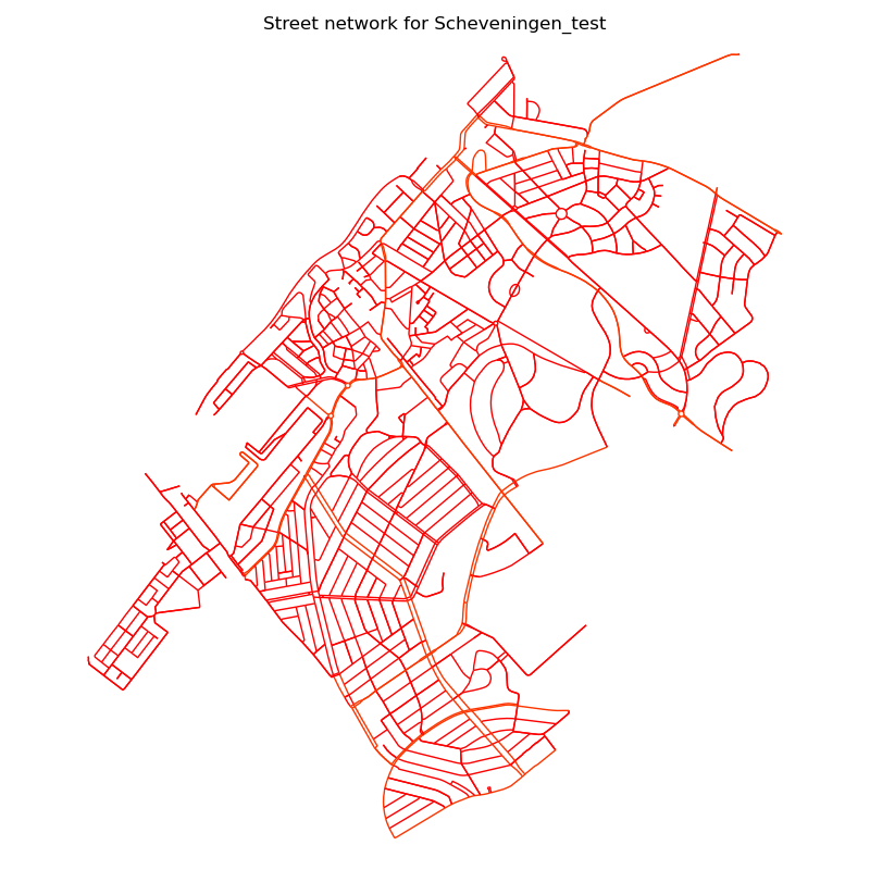
Street network of Scheveningen — Simple street network of Scheveningen.#

First, you want to see the street network of the city you are working with. This should look like the street network of the place you want to analyze, if it does not, check the search_str or the OSM relation ID. Some streets at the outer edges might be cut off, this is due to the requirement that the street network needs to be strongly connected, in other words, you should be able to reach every street from every other street. For in- and outgoing highways, this might not be the case, so they are cut off. Furthermore, the network filter decides which streets are included in the start.

Component rank size plot for street length of Superblocks — Superblock street length rank size plot.#

Generally, a rank-size plot shows the distribution of a quantity in descending order. In this case, the street length of the generated Superblocks is shown on a logaritmic scale. If you are more interested in the tesselated Superblock areas, instead of the street length, you can find this information in the geopackage file saved later.

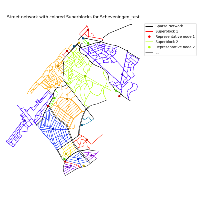
Superblocks of Scheveningen — Generated Superblocks for Scheveningen. Each Superblock is colored differently with one representative point for visual aid.#

A central feature of this package is the distance calculation between every point on the map before \(d_S(i,j)\) and after introducing the Superblocks \(d_N(i,j)\). This is done to evaluate the generated Superblock configuration. The way the distance calculation works is explained in the Restricted Distance Calculation section. The restriction imposed by the Superblocks is that after implementing them, one is not allowed to travel through a Superblock that does not contain the starting or ending point. Another visualization of this restriction is shown on the Betweenness Centrality explainer page.

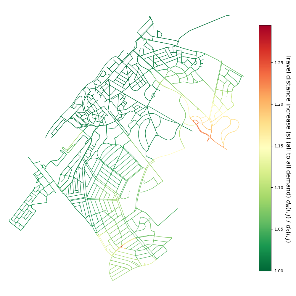
Relative increase of the distance metric on the graph.#

The fraction of the two distances \(d_N(i,j)/d_S(i,j)\) is shown on the street network. If this is close to \(1\), the Superblocks do not restrict the travel distance much. A value of \(1.1\) means that the travel distance is increased by \(10\%\). As we specified the unit as “time” in the initialization (unit="time"), the distance metric is in minutes and one can talk about a \(10\%\) increase in travel time.

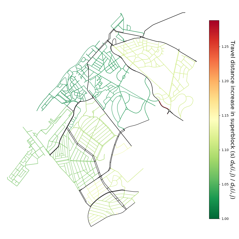
Component-wise travel increase — Travel increase for each Superblock.#

Finally, the travel increase is shown as arithmetic mean for each Superblock.

All shown plots are saved as pdf to the data/results/Scheveningen_test folder. Here, is possible to save and load a partitioner object to continue the work later.

part.save()
part.load("Scheveningen_test")

The most illustrative and interactive way to view the results is to save them to a geopackage file. This file can be opened in QGIS and edited further.

sb.save_to_gpkg(part, save_path=None)

2024-12-04 10:45:49,151 |     INFO | utils.py:102 | Using components attribute to save Superblocks to geodatapackage /home/runner/work/superblockify/superblockify/docs/data/results/Scheveningen_test/Scheveningen_test.gpkg

2024-12-04 10:45:49,206 |     INFO | utils.py:148 | Node attributes: Index(['y', 'x', 'street_count', 'node_betweenness_normal',
       'node_betweenness_length', 'node_betweenness_linear',
       'node_betweenness_normal_restricted',
       'node_betweenness_length_restricted',
       'node_betweenness_linear_restricted', 'representative_node_name',
       'split', 'geometry'],
      dtype='object')

2024-12-04 10:45:49,207 |     INFO | utils.py:149 | Edge attributes: Index(['osmid', 'highway', 'length', 'bearing', 'speed_kph', 'travel_time',
       'population', 'area', 'cell_id', 'residential',
       'travel_time_restricted', 'component_name', 'edge_betweenness_normal',
       'edge_betweenness_length', 'edge_betweenness_linear',
       'edge_betweenness_normal_restricted',
       'edge_betweenness_length_restricted',
       'edge_betweenness_linear_restricted', 'rel_increase',
       'rel_increase_comp', 'classification', 'geometry'],
      dtype='object')

2024-12-04 10:45:49,207 |     INFO | utils.py:150 | Superblock attributes: Index(['classification', 'value', 'm', 'n', 'length_total', 'ignore',
       'representative_node_id', 'mean_edge_betweenness_normal',
       'mean_edge_betweenness_length', 'mean_edge_betweenness_linear',
       'mean_edge_betweenness_normal_restricted',
       'mean_edge_betweenness_length_restricted',
       'mean_edge_betweenness_linear_restricted',
       'change_mean_edge_betweenness_normal',
       'change_mean_edge_betweenness_length',
       'change_mean_edge_betweenness_linear', 'population', 'area',
       'population_density', 'k_avg', 'edge_length_total', 'edge_length_avg',
       'streets_per_node_avg', 'streets_per_node_counts',
       'streets_per_node_proportions', 'intersection_count',
       'street_length_total', 'street_segment_count', 'street_length_avg',
       'circuity_avg', 'self_loop_proportion', 'node_density_km',
       'intersection_density_km', 'edge_density_km', 'street_density_km',
       'street_orientation_order', 'representative_node_point'],
      dtype='object')

2024-12-04 10:45:49,208 |     INFO | utils.py:151 | Graph meta attributes: Index(['created_date', 'created_with', 'crs', 'simplified', 'edge_population',
       'boundary_crs', 'boundary', 'area', 'n', 'm', 'k_avg',
       'edge_length_total', 'edge_length_avg', 'streets_per_node_avg',
       'streets_per_node_counts', 'streets_per_node_proportions',
       'intersection_count', 'street_length_total', 'street_segment_count',
       'street_length_avg', 'circuity_avg', 'self_loop_proportion',
       'node_density_km', 'intersection_density_km', 'edge_density_km',
       'street_density_km', 'street_orientation_order'],
      dtype='object')

2024-12-04 10:45:49,235 |     INFO | raw.py:723 | Created 995 records

2024-12-04 10:45:49,238 |     INFO | utils.py:171 | Saved 995 nodes to /home/runner/work/superblockify/superblockify/docs/data/results/Scheveningen_test/Scheveningen_test.gpkg

2024-12-04 10:45:49,274 |     INFO | raw.py:723 | Created 2,307 records

2024-12-04 10:45:49,284 |     INFO | utils.py:173 | Saved 2307 edges to /home/runner/work/superblockify/superblockify/docs/data/results/Scheveningen_test/Scheveningen_test.gpkg

2024-12-04 10:45:49,291 |     INFO | raw.py:723 | Created 26 records

2024-12-04 10:45:49,299 |     INFO | utils.py:175 | Saved 26 Superblocks to /home/runner/work/superblockify/superblockify/docs/data/results/Scheveningen_test/Scheveningen_test.gpkg

2024-12-04 10:45:49,305 |     INFO | raw.py:723 | Created 6 records

2024-12-04 10:45:49,312 |     INFO | utils.py:177 | Saved graph meta to /home/runner/work/superblockify/superblockify/docs/data/results/Scheveningen_test/Scheveningen_test.gpkg

This will save the partitioning results to data/results/Scheveningen_test/{city_name}.gpkg. If you calculated the metrics before, they will be available in the layers, for each Superblock. This includes more metrics than shown in the plots earlier. The name of the components is saved into a classification edge attribute. The sparse graph is saved with the value “SPARSE” into the classification edge attribute.

To learn more about the inner workings and background of the package, please see the next Reference section. Otherwise, you can also check out the API documentation.

FAQ#

Can I export the plots to another format?#

Yes, you can export the plots to any format supported by matplotlib. Just change the PLOT_SUFFIX attribute in the Config class to the desired format.

sb.config.Config.PLOT_SUFFIX = "png"  # or "svg", "pdf", etc.

The downloaded city is too big/small/not the right city, can I change this?#

The deciding string for the area to download is the search_str. Finding a fitting OSM area is via the Nominatim API. If you want to see your area before downloading, use the Nominatim Search. It helps to be more specific, e.g. “Scheveningen, The Hague, Netherlands” instead of just “Scheveningen”. Otherwise, OSM relations IDs, e.g. R13751467, can be used.

To re-download the map, pass reload_graph=True when initializing the partitioner.

part = sb.ResidentialPartitioner(
    name="Scheveningen_test",
    ...,
    reload_graph=True,
)

The Superblocks look too big/small/random when using the `ResidentialPartitioner`, why is that?#

The ResidentialPartitioner uses the residential street tags to find the Superblocks. The variation in OSM data quality and street tagging practices can be reflected when using this approach. The BetweennessPartitioner instead does not rely on OSM tags but uses the betweenness centrality - a topological property of the street network. Try this approach if the Superblocks from the ResidentialPartitioner are not satisfactory .

superblockify.partitioning.approaches.betweenness.BetweennessPartitioner(name='unnamed', city_name=None, search_str=None, unit='time', graph=None, reload_graph=False, max_nodes=20000)[source]

Partitioner using betweenness centrality of nodes and edges.

Set sparsified graph from edges or nodes with high betweenness centrality.

superblockify.partitioning.approaches.betweenness.BetweennessPartitioner.write_attribute()

Determine edges with high betweenness centrality for sparsified graph.

Edges with high betweenness centrality are used to construct the sparsified graph.

The high percentile is determined through ranking all edges by their betweenness centrality and taking the top percentile. The percentile is determined by the percentile parameter.

Parameters:

percentilefloat, optional: The percentile to use for determining the high betweenness centrality edges, by default 90.0
scalingstr, optional: The type of betweenness to use, can be normal, length, or linear, by default normal
max_rangeint, optional: The range to use for calculating the betweenness centrality, by default None, which uses the whole graph. Its unit is meters.
**kwargs: Additional keyword arguments. calculate_metrics_before takes the make_plots parameter.

Raises:

ValueError: If scaling is not normal, length, or linear.
ValueError: If percentile is not between, 0.0 and 100.0.

Pass the kwargs from the write_attribute() method (as seen above or in the API documentation) to the BetweennessPartitioner.run(...) method to set the parameters for the partitioning. After initializing a BetweennessPartitioner, part = BetweennessPartitioner(...), run the partitioning with the optional parameters, e.g. part.run(percentile=85.0, scaling="normal", max_range=None).

My country has another maximum speed limit, can I change this?#

When calculating the metrics and using replace_max_speeds=True, the maximum speed limits are set to 15 km/h inside the Superblocks and 50 km/h outside of them. If you want to change these values, you can do so by setting the V_MAX_LTN and V_MAX_SPARSE attributes in the Config class.

sb.config.Config.V_MAX_LTN = 30  # km/h
sb.config.Config.V_MAX_SPARSE = 60  # km/h

Some streets I know are not being used in the partitioning, why is that?#

When downloading the map from OpenStreetMap, we use a specific network filter, which should include the car network.

sb.config.Config.NETWORK_FILTER

'["highway"]["area"!~"yes"]["access"!~"private"]["highway"!~"abandoned|bridleway|bus_guideway|busway|construction|corridor|cycleway|elevator|escalator|footway|path|pedestrian|planned|platform|proposed|raceway|service|steps|track"]["motor_vehicle"!~"no"]["motorcar"!~"no"]["service"!~"alley|driveway|emergency_access|parking|parking_aisle|private"]'

If you want to include more streets, you can change the network filter to include more or less streets. When changing the network filter, you might want to remove the cached graphs, or set reload_graph=True when initializing the partitioner.

Some process is taking too long or suddenly stops, what can I do?#

If there are warnings or logs that indicate a problem, they might point to the issue. Be aware that, when analyzing a large city, superblockify needs sufficient resources. If it runs out of memory, some processes might stop abruptly without warning. To combat this, you can either try to find a search_str with a smaller area or set the MAX_NODES attribute in the Config class to a lower value. When initializing a partitioner, the street network is cut off at this number of nodes, including the most central nodes. By default, this is set to 20,000.

For further settings, see the other attributes in the Config class.

superblockify.config.Config()[source]

Configuration class for superblockify.

Attributes:

WORK_DIR: The working directory of the package. This is used to store the graphs and results in subdirectories of this directory. By default, this is the current working directory when the package is imported. This is only used to define the following directories.
GRAPH_DIR: The directory where the graphs are stored.
RESULTS_DIR: The directory where the results are stored.
GHSL_DIR: The directory where the GHSL population data is stored when downloaded.
V_MAX_LTN: The maximum speed in km/h for the restricted calculation of travel times.
V_MAX_SPARSE: The maximum speed in km/h for the restricted calculation of travel times for the sparsified graph.
NETWORK_FILTER: The filter used to filter the OSM data for the graph. This is a string that is passed to the osmnx.graph_from_place() function.
CLUSTERING_PERCENTILE: The percentile used to determine the betweenness centrality threshold for the spatial clustering and anisotropy nodes.
NUM_BINS: The number of bins used for the histograms in the entropy calculation.
FULL_RASTER: The path and filename of the full GHSL raster. If None, tiles of the needed area are downloaded from the JRC FTP server and stored in the GHSL_DIR directory. <https://jeodpp.jrc.ec.europa.eu/ftp/jrc-opendata/GHSL/GHS_POP_GLOBE_R2023A/GHS_POP_E2025_GLOBE_R2023A_54009_100/V1-0/GHS_POP_E2025_GLOBE_R2023A_54009_100_V1_0.zip>
DOWNLOAD_TIMEOUT: The timeout in seconds for downloading the GHSL raster tiles.
logger: The logger for this module. This is used to log information, warnings and errors throughout the package.
TEST_DATA_PATH: The path to the test data directory.
HIDE_PLOTS: Whether to hide the plots in the tests.
PLACES_GENERAL: A list of tuples of the form (name, place) where name is the name of the place and place is the place string that is passed to the superblockify.utils.load_graph_from_place() function.
PLACES_SMALL: Same as PLACES_GENERAL but for places of which the graph is small enough to be used in the tests.
PLACES_100_CITIES: 100 cities from Boeing et al. (2019) <https://doi.org/10.1007/s41109-019-0189-1> A dictionary of the form {name: place} where name is the name of the place, and place is a dictionary of various attributes. One of them is the query attribute which is the place string or a list of place strings. Find the extensive list in the ./cities.yml file.
PLACES_GERMANY: List of cities in Germany by population. All cities with more than 100,000 inhabitants are included. Data from the German Federal Statistical Office.
PLOT_SUFFIX: The format of the plots. Can be "png", "jpg", "pdf", "svg", etc. Matplotlib uses the Pillow library to save the plots, so all formats supported by Pillow are supported by Matplotlib. <https://pillow.readthedocs.io/en/stable/handbook/image-file-formats.html>
MAX_NODES: The maximum number of nodes in the graph. If the graph has more nodes, it is reduced. See superblockify.partitioning.utils.reduce_graph().

If you run into any other issues, feel free to look into the API documentation, Source Code, activate debug logs sb.config.set_log_level("DEBUG") or finally open a new issue.

Usage

Contents